SQL

Phase 1 – Foundation: How Data & Databases Work

Phase 1 Overview

#	Subtopic	Learning Outcome
1	Introduction to Data	Data types, data vs. information, and storage methods
2	Introduction to Servers	Client-server model and request-response flow
3	Introduction to Databases	Why organizations use databases over files/spreadsheets
4	DBMS	Core responsibilities: storage, retrieval, security, integrity, backup
5	DBMS Architecture	1-tier, 2-tier, and 3-tier system design
6	Types of Databases	Relational, NoSQL, Cloud, OLTP, and OLAP

Module 1: Introduction to Data

1.1 What Is Data?

Data is a collection of raw facts, figures, or symbols recorded for reference. It can be numeric, textual, visual, or sensory — a salary figure, a city name, a photograph, a temperature reading taken every second.

The defining characteristic of data is that it carries no meaning on its own. The value 45000 could be a salary, a population, a part number, or a distance in metres. Nothing about the value itself tells you which.

Raw: it has not been processed, cleaned, or interpreted.
Context-free: it does not say what it measures or which entity it belongs to.
Not actionable: no decision can responsibly be made from it as it stands.
Independent: it exists whether or not anyone ever uses it.

Example: 1023, Ravi, 45000, Sales — four values sitting in a row, meaning nothing yet.

1.2 What Is Information?

Information is data that has been processed, organized, and placed in context so that it answers a question. The values are the same; what changes is that each one has been given a role, a unit, and a relationship to the others.

Processed: cleaned, aggregated, or otherwise transformed.
Contextual: each value is tied to what it measures and whom it describes.
Meaningful: it answers a specific question someone actually asked.
Actionable: a decision can be based on it.
Derived: it cannot exist without underlying data.

Example: "Employee 1023, Ravi, earns ₹45,000 per month in the Sales department." The same four values now support a payroll or headcount decision.

1.3 Data vs. Information Compared

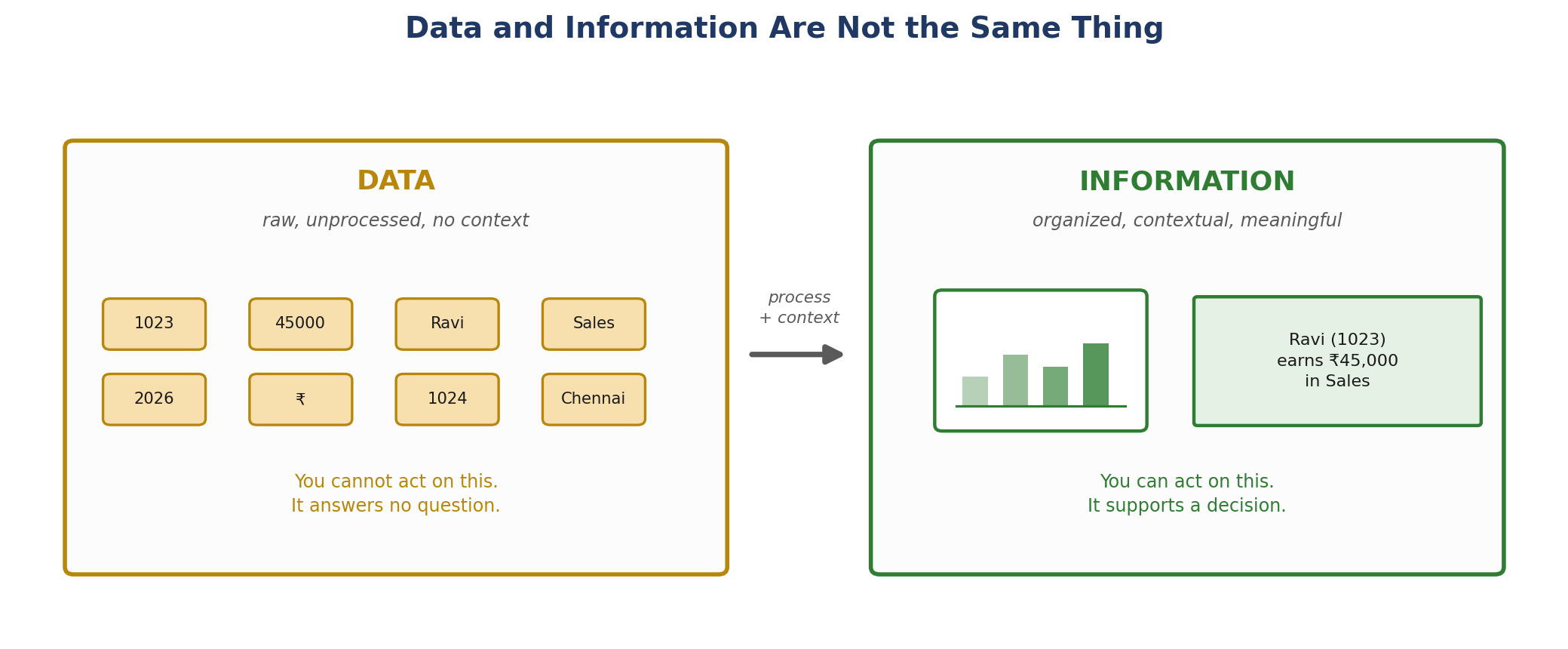
Data and information are not the same thing

Figure 1.1 — The same values before and after context is applied.

Aspect	Data	Information
Definition	Raw, unprocessed facts	Processed, organized, contextual data
Meaning	None on its own	Carries meaning
Dependency	Exists independently	Derived from data
Usability	Not actionable	Supports a decision
Form	Values, symbols, readings	Reports, summaries, statements
Example	1023, Ravi, 45000, Sales	Ravi (1023) earns ₹45,000 in Sales

Put simply: Information = Data + Context + Processing + Interpretation. Every analytics task is some version of moving from the left column to the right one.

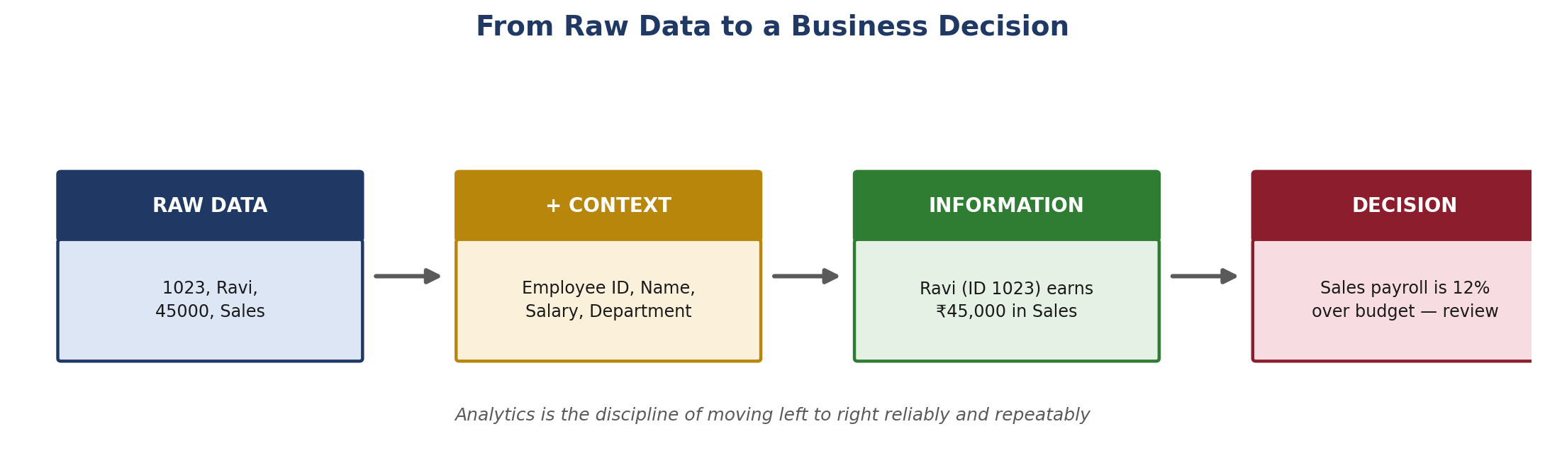
Figure 1.2 — The full path from raw values to a decision.

1.4 The Three Structural Categories

Structure determines which tools can touch the data, which query language applies, and how much preprocessing is required before analysis.

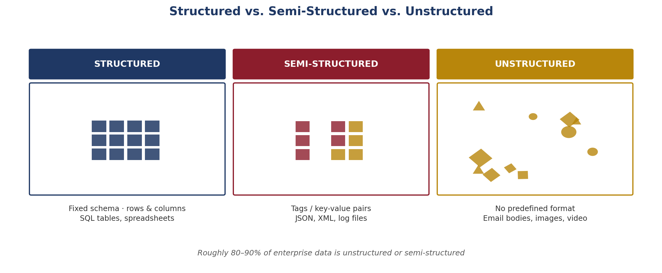
Structured vs semi-structured vs unstructured

Figure 1.3 — The three structural categories.

	Structured	Semi-Structured	Unstructured
Schema	Fixed, defined upfront	Flexible, self-describing	None
Format	Rows and columns	JSON, XML, logs	Text, image, audio, video
Queried with	SQL	Document queries, path expressions	NLP, computer vision, embeddings
Stored in	RDBMS, warehouses	NoSQL, data lakes	Object storage, data lakes

A practical nuance: the boundary is about how the data is used, not where it sits. A CSV column containing nested JSON strings is semi-structured despite living in a tabular file. An email is semi-structured if you treat its headers as fields, and unstructured if you need meaning from its body.

1.5 Where Data Is Stored

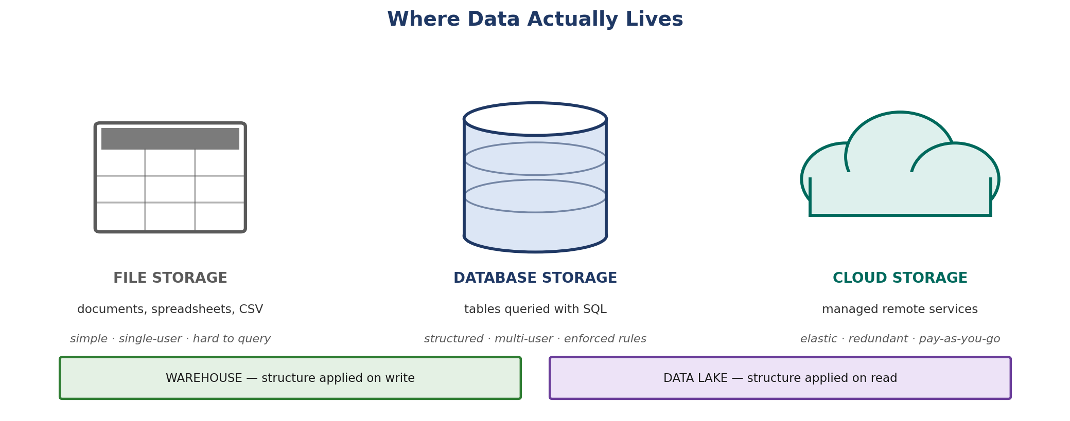
Figure 1.4 — The storage landscape, from files to lakes.

The warehouse-versus-lake distinction matters most in practice. A warehouse enforces structure on write, so data arrives clean and query-ready. A lake accepts anything and applies structure on read, which preserves flexibility but shifts the cleaning burden onto whoever queries it.

Best Practice: Classify data by structure and business usage, not by file extension.

Module 2: Introduction to Servers

2.1 What a Server Actually Is

A server is a program that waits for requests and responds to them. It is a role, not a box: one machine can run several server processes, and one logical service can span many machines.

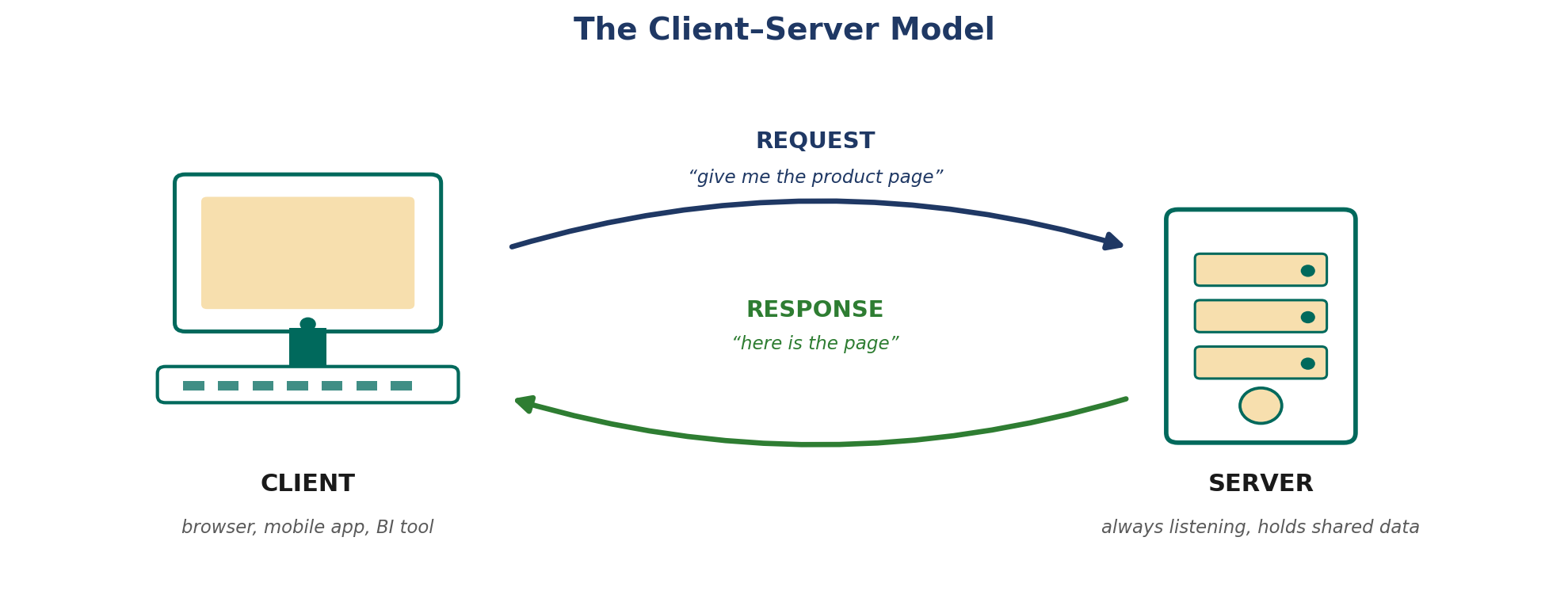
Figure 2.1 — Many clients, one shared server.

2.2 The Three Servers Behind a Web Application

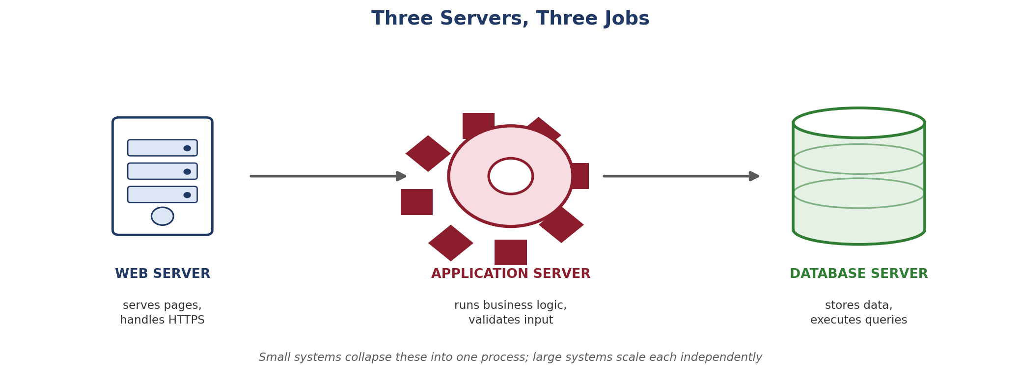
Figure 2.2 — Web, application, and database servers.

The application server holds business rules; the database server holds state. Keeping them distinct is what allows logic to be changed without touching storage, and storage to be scaled without rewriting logic.

	Application Server	Database Server
Holds	Business logic	Persistent data
Talks to	Clients and the database	Application servers only
Scales by	Adding instances (horizontal)	Bigger machine, then replicas/shards
Example work	Validate a discount code	Execute a JOIN across two tables

2.3 The Request–Response Cycle

Every interaction follows the same shape: the client asks, the server coordinates work, the response returns along the same path. Reading this as a sequence over time makes the dependencies explicit.

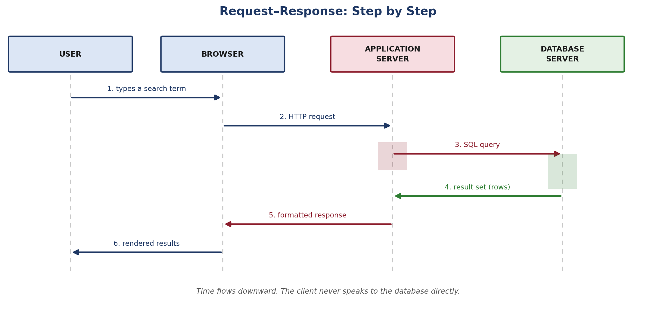
Figure 2.3 — A search request as a time sequence.

Two details worth noticing. The database is only busy during step 3–4, so a slow report holds that resource against everyone else. And the browser never holds database credentials — the application server is the only component that does.

Best Practice: Keep client, application, and database responsibilities clearly separated.

Hands-On: Draw the flow of an e-commerce search: User → Browser → Application Server → Database Server → Application → User. Label every arrow with what is actually being sent (search term, HTTP request, SQL query, result set, rendered page, displayed result).

Module 3: Introduction to Databases

3.1 Why Files and Spreadsheets Fail at Scale

Spreadsheets work until more than one person needs the same truth at the same time. Then the failure modes arrive together.

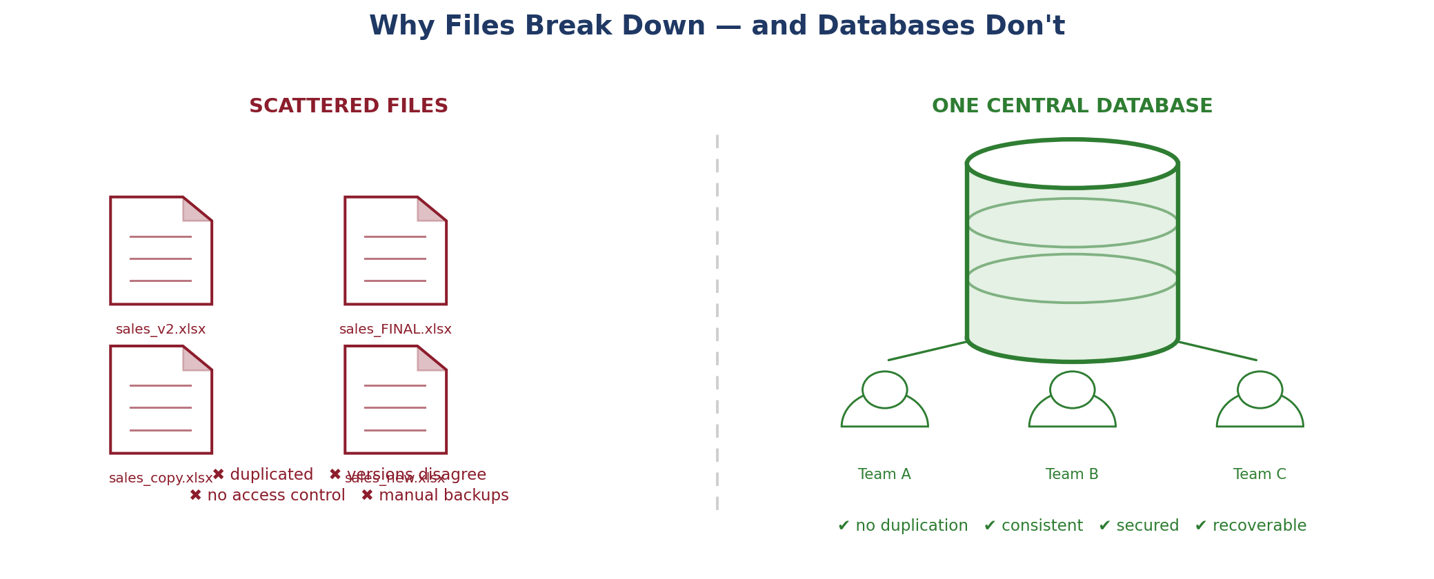
Why files break down and databases don't

Figure 3.1 — The same data, managed two ways.

	Files / Spreadsheets	Database
Redundancy	Copies multiply silently	Minimized by design (normalization)
Consistency	Versions drift apart	One authoritative value
Concurrency	Overwrites and conflicts	Managed by transactions and locks
Security	File-level password at best	Row- and column-level permissions
Recovery	Whatever was last copied	Point-in-time restore from logs

3.2 How a Table Is Built

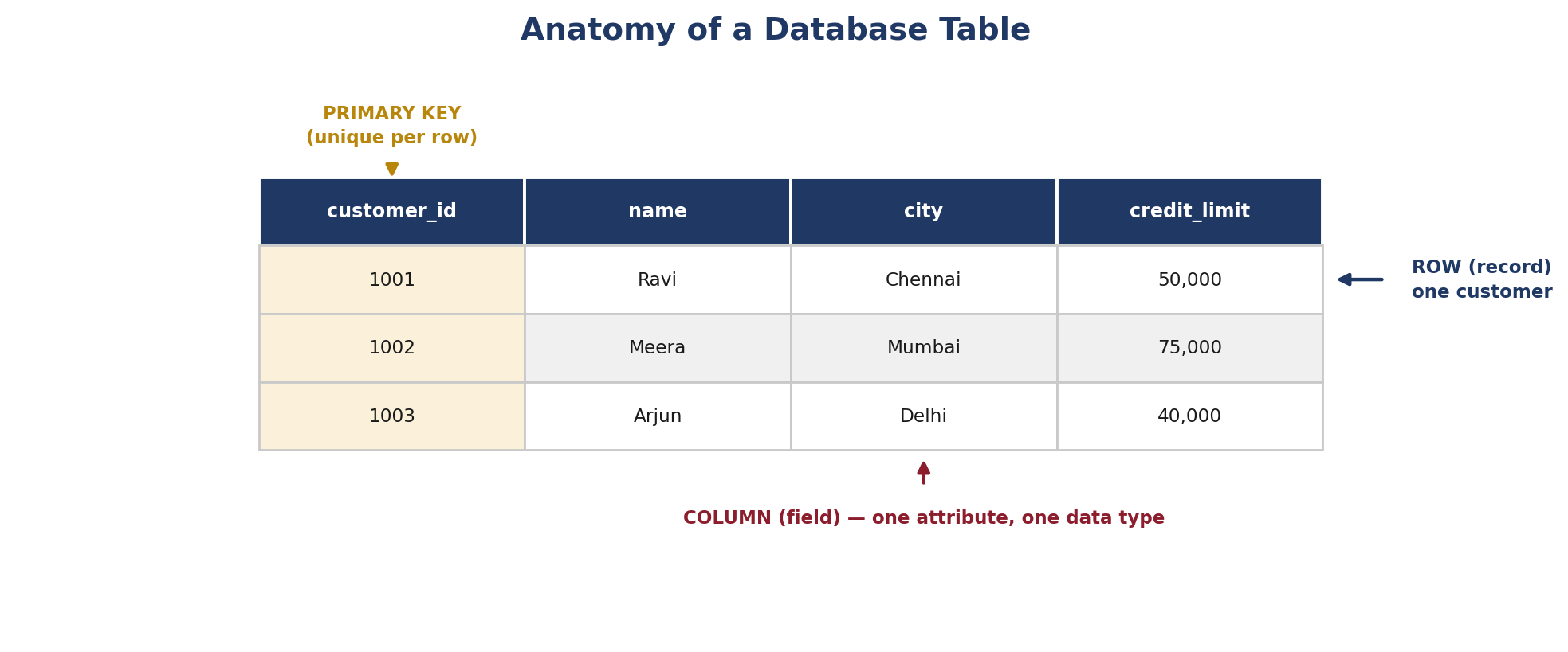
Figure 3.2 — Rows, columns, and the primary key.

Column: one attribute, one data type, applied to every row.
Row: one complete record — one customer, one order, one event.
Primary key: the column whose value uniquely identifies a row and is never duplicated or empty.

3.3 Relationships Are the Real Advantage

Storing data once and linking to it is what removes duplication. A foreign key points from one table to another table's primary key, and the database enforces that the target actually exists.

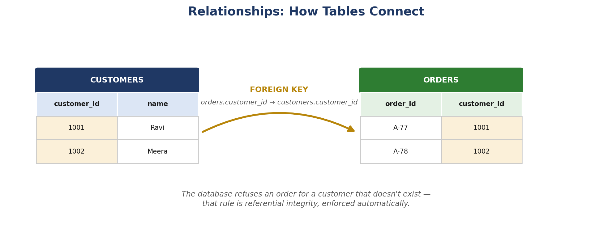
Figure 3.3 — A foreign key linking orders to customers.

This is why a customer's address is stored in one place rather than repeated on every order. Change it once and every related record reflects it immediately — no reconciliation, no stale copies.

Best Practice: Avoid unnecessary duplication and keep storage centralized.

Module 4: DBMS – Database Management System

4.1 The DBMS as an Abstraction Layer

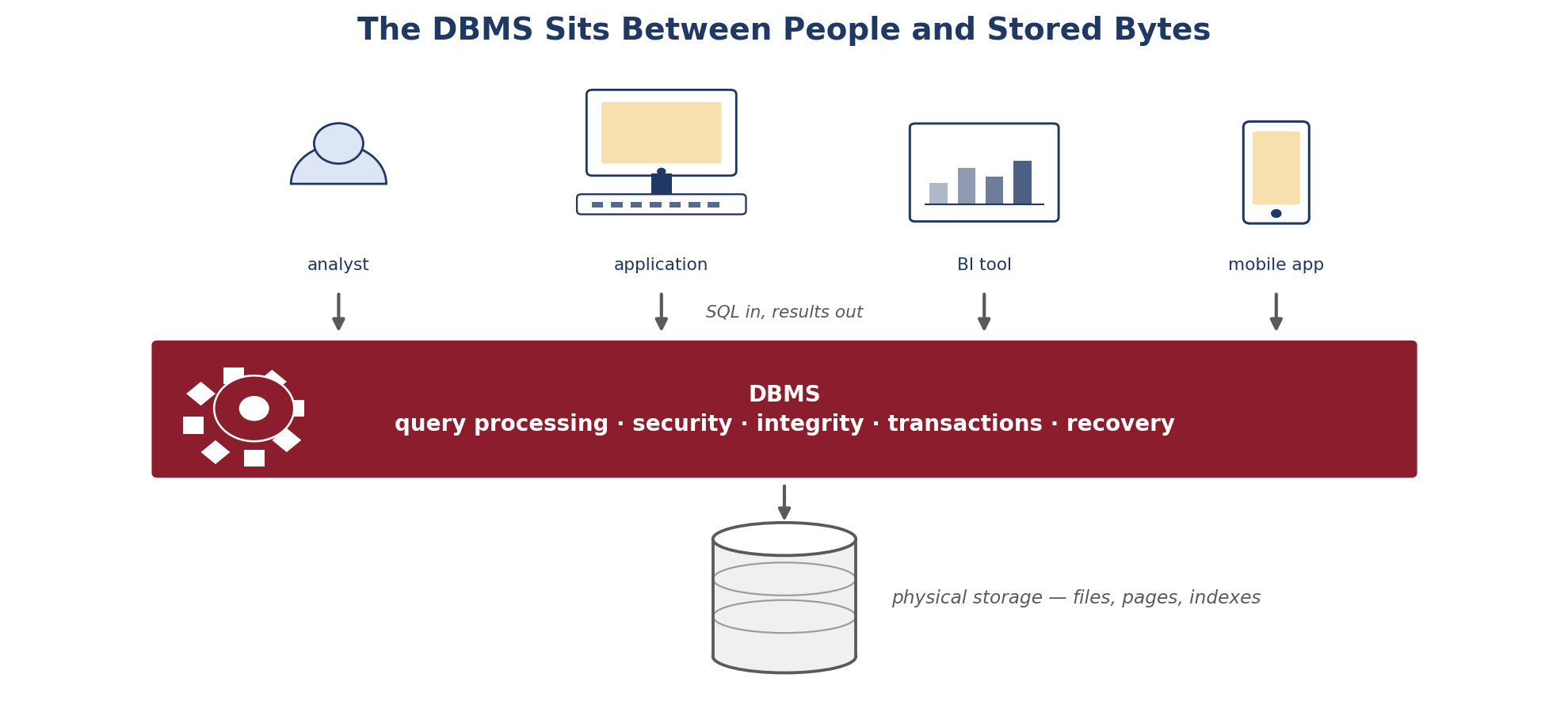
The DBMS sits between people and stored bytes

Figure 4.1 — The DBMS sits between people and physical storage.

Nobody writing a query needs to know which disk block holds a row. That separation — data independence — is what lets storage be reorganized without rewriting a single query.

4.2 What the DBMS Is Responsible For

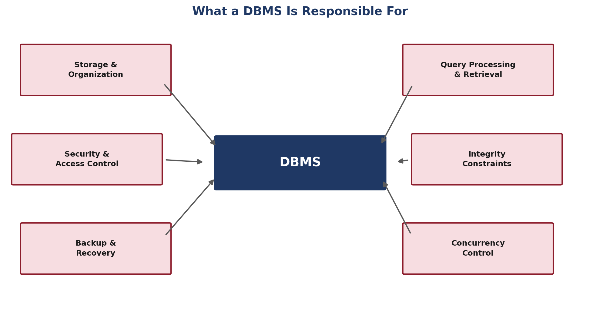
Figure 4.2 — Six responsibilities, all handled centrally.

Storage & organization: mapping logical tables onto physical pages and indexes.
Query processing: parsing SQL, choosing an execution plan, returning results.
Security: authenticating users and enforcing what each may read or write.
Integrity: rejecting data that violates keys, types, or constraints.
Backup & recovery: restoring to a consistent state after failure using transaction logs.
Concurrency control: letting many users work at once without corrupting each other's results.

4.3 Transactions and ACID

A transaction is a unit of work that must succeed or fail as a whole. ACID names the four guarantees that make this dependable.

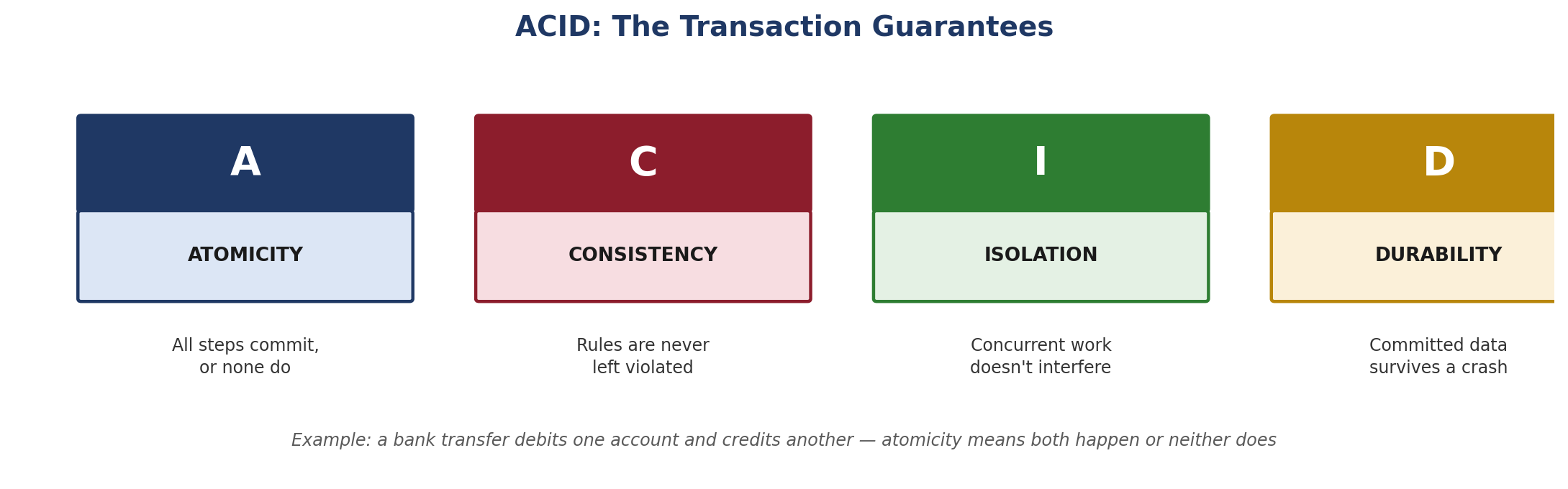
Figure 4.3 — The four transaction guarantees.

4.4 How a Query Is Answered

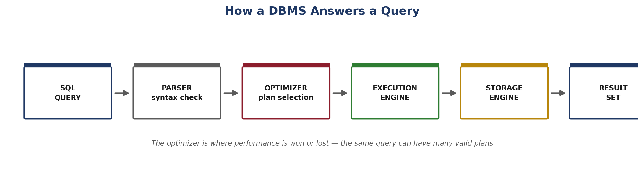
Figure 4.4 — From SQL text to result set.

The optimizer is the component analysts feel most. SQL declares what is wanted, not how to get it, so the same query can be executed many different ways — and the plan chosen is usually the difference between two seconds and two minutes.

Best Practice: Choose a DBMS on requirements, not familiarity.

Module 5: DBMS Architecture

5.1 One, Two, and Three Tiers

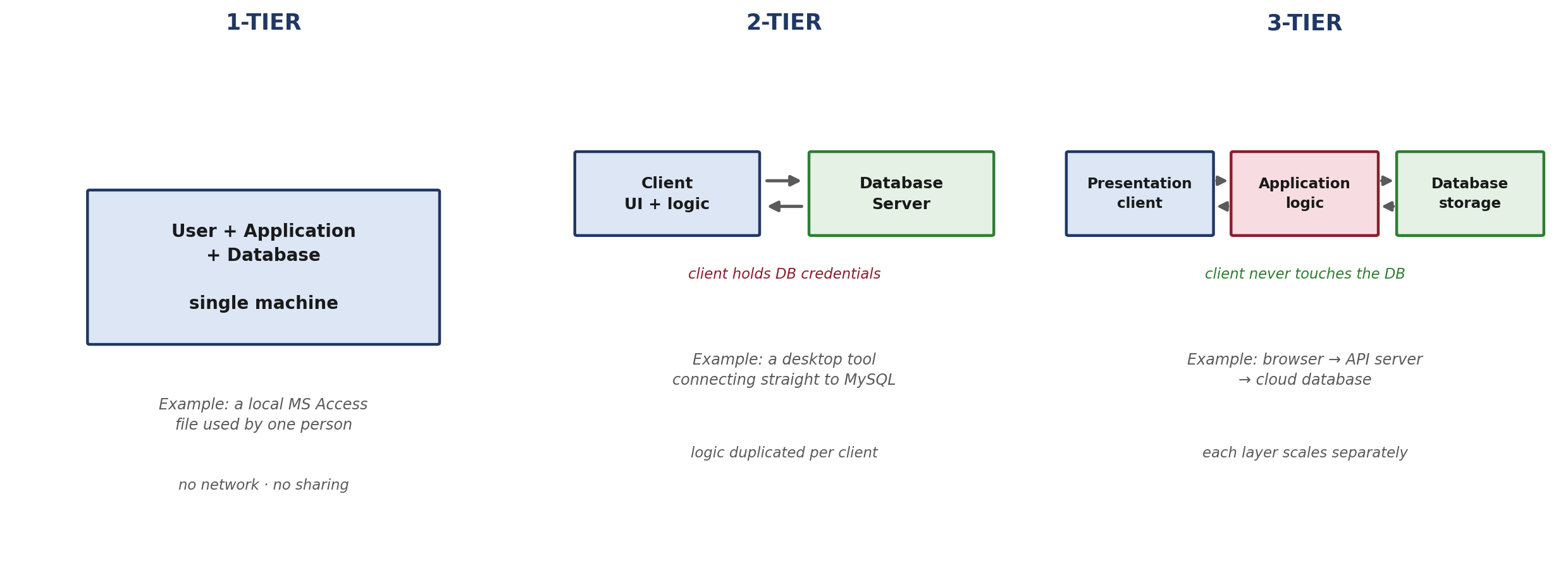
Figure 5.1 — The three architectural patterns.

	1-Tier	2-Tier	3-Tier
Layout	Everything on one machine	Client → database	Client → application → database
Users	One	Small team	Enterprise / public
Business logic	In the single app	Duplicated in each client	Centralized in one layer
DB credentials	Local	Held by every client	Held only by the app layer
Scalability	None	Limited	Each layer scales alone

The decisive difference is the credential row. In 2-tier, every client machine can reach the database directly, so a compromised laptop is a compromised database. In 3-tier, the database only ever accepts connections from the application layer.

5.2 The Three-Schema Architecture

Separate from tiers, a DBMS also layers its own view of the data into three levels. This is what makes physical change safe.

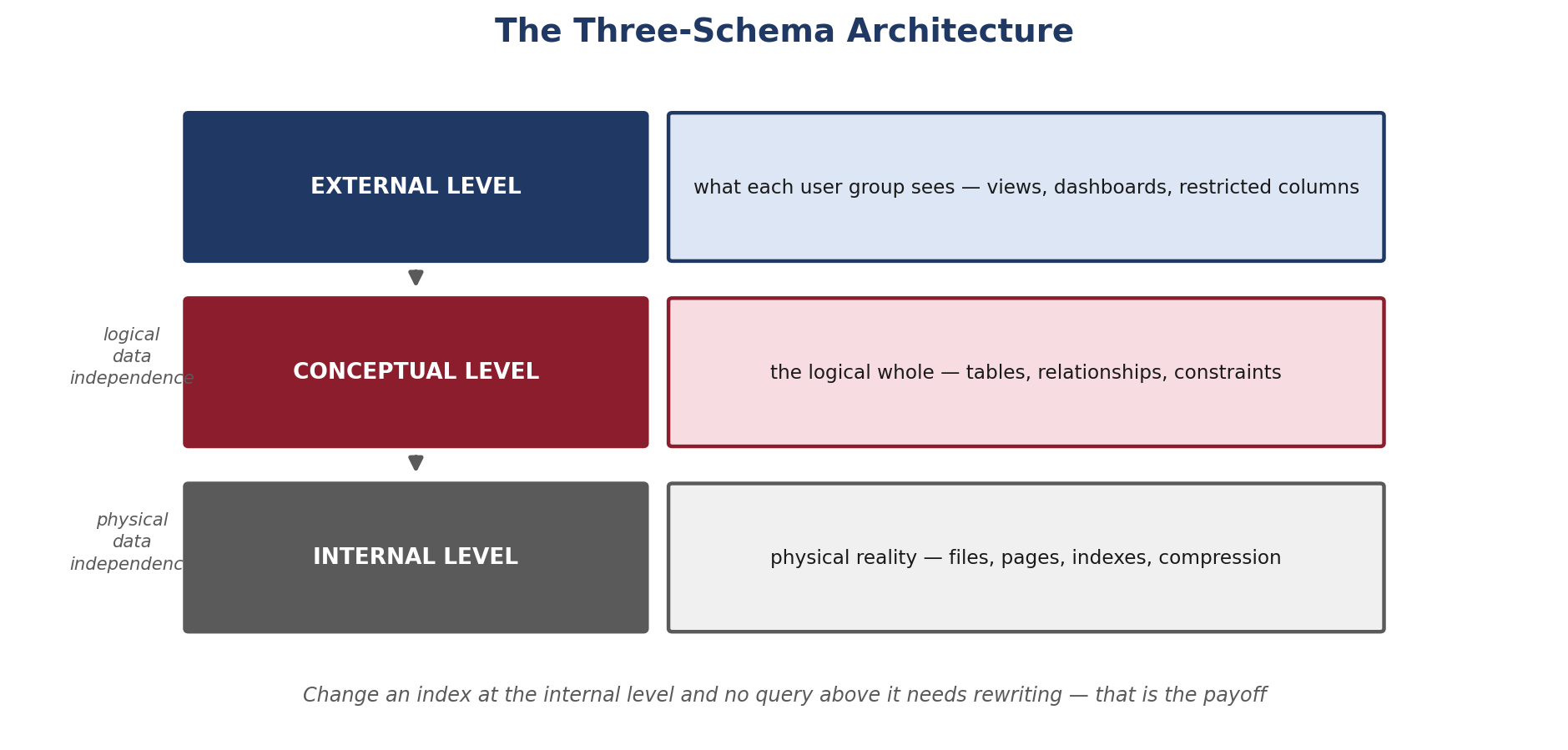
Figure 5.2 — External, conceptual, and internal levels.

Logical data independence: add a column at the conceptual level without breaking existing user views.
Physical data independence: add an index or repartition storage without changing a single query.

Best Practice: Prefer layered architecture for enterprise applications.

Hands-On: Draw 1-tier, 2-tier, and 3-tier diagrams with a real example for each — for instance a personal budgeting app, a clinic's desktop appointment system, and an online banking portal. Label every component and the direction of each connection.

Module 6: Types of Databases

6.1 The Landscape

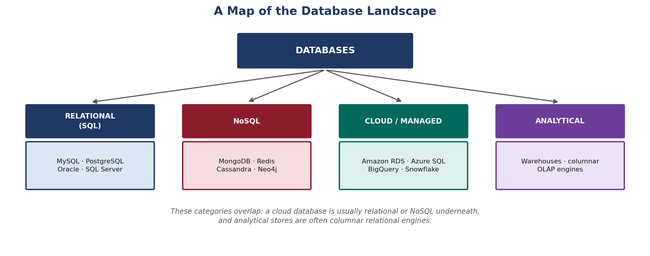
Figure 6.1 — How the categories relate.

These categories overlap deliberately. A cloud database is relational or NoSQL underneath; an analytical store is usually a columnar relational engine. The labels describe emphasis, not mutually exclusive families.

6.2 Relational Databases

Data lives in tables with a schema defined before insertion, related through keys, queried with SQL, and protected by ACID guarantees. This remains the default choice whenever correctness matters more than flexibility — finance, orders, inventory, records.

Examples: MySQL, PostgreSQL, Oracle Database, Microsoft SQL Server.

6.3 NoSQL Databases

NoSQL covers four distinct models that share one trait: they relax the fixed relational schema to gain flexibility or horizontal scale.

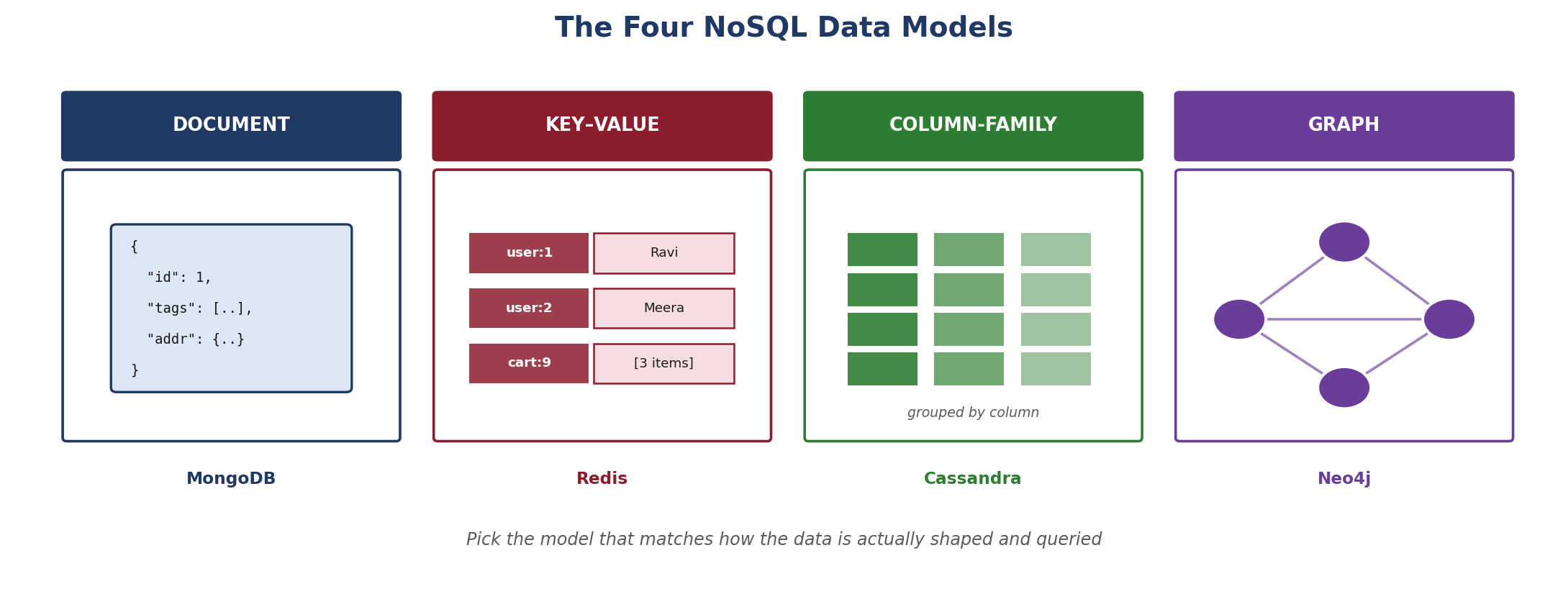
Figure 6.2 — The four NoSQL data models.

Document: nested, self-contained records where fields vary between entries — catalogs, user profiles, content.
Key-value: the fastest possible lookup by identifier — caching, sessions, feature flags.
Column-family: wide, sparse tables distributed across many machines — time series, event logs at scale.
Graph: relationships stored as first-class objects — fraud rings, recommendations, network analysis.

6.4 Cloud Databases

A cloud database is a managed service rather than a distinct data model. The provider handles provisioning, patching, replication, and backups; the organization trades some control and predictable cost for a large reduction in operational work. Examples: Amazon RDS and Aurora, Azure SQL Database, Google BigQuery, Snowflake.

6.5 OLTP — Online Transaction Processing

An OLTP system is the database behind the software that runs the business as it happens. Every time an order is placed, a seat is booked, a payment clears, or a password is changed, an OLTP database records it.

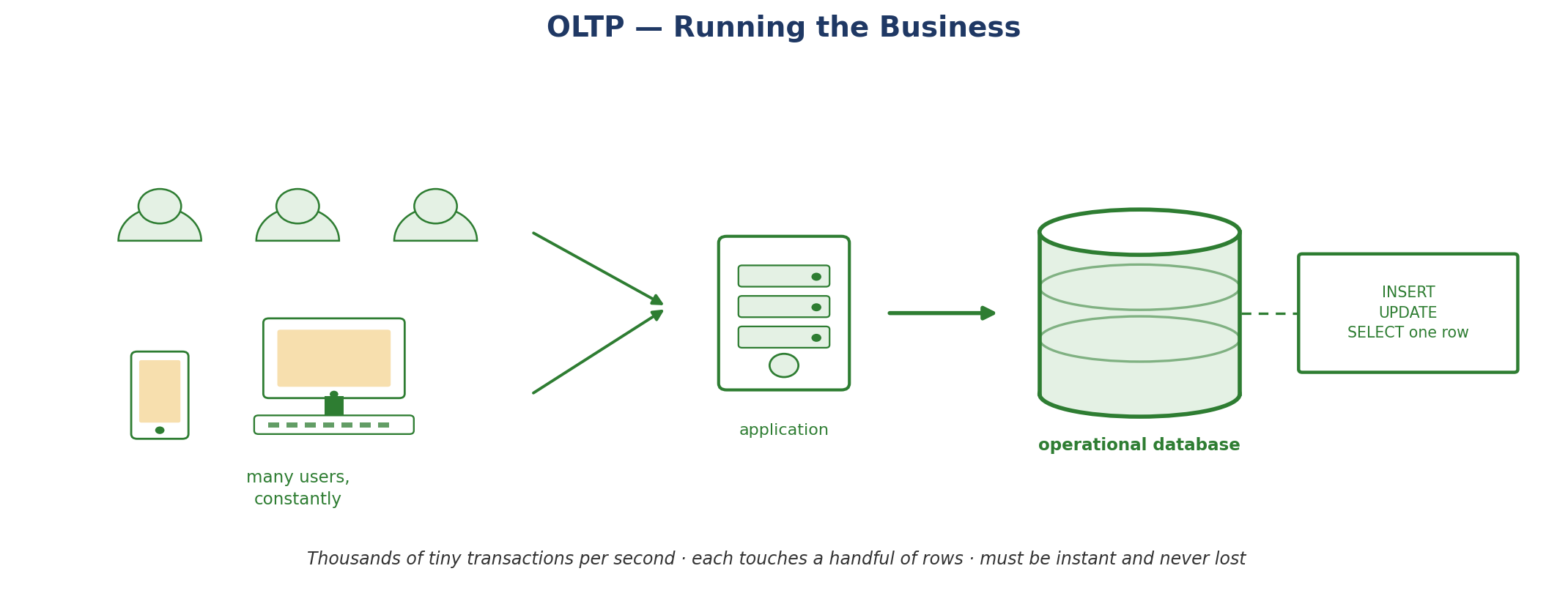
Figure 6.3 — An OLTP system under normal load.

Characteristics

Workload: a very high volume of small, short-lived transactions — inserts, updates, and single-record reads.
Rows touched: one to a few per operation.
Priority: low latency and absolute correctness; a lost order is unacceptable.
Data held: current operational state, typically normalized to avoid duplication.
Concurrency: thousands of users writing simultaneously, coordinated by ACID transactions.
Storage layout: row-oriented, so a whole record is retrieved in one read.

Typical systems: MySQL, PostgreSQL, Oracle Database, Microsoft SQL Server. Typical uses: e-commerce checkout, core banking, ticket booking, inventory, CRM.

6.6 OLAP — Online Analytical Processing

An OLAP system exists to answer questions about the business rather than to run it. It holds history, organized so that large-scale aggregation is fast: revenue by region by quarter, churn by cohort, year-on-year growth.

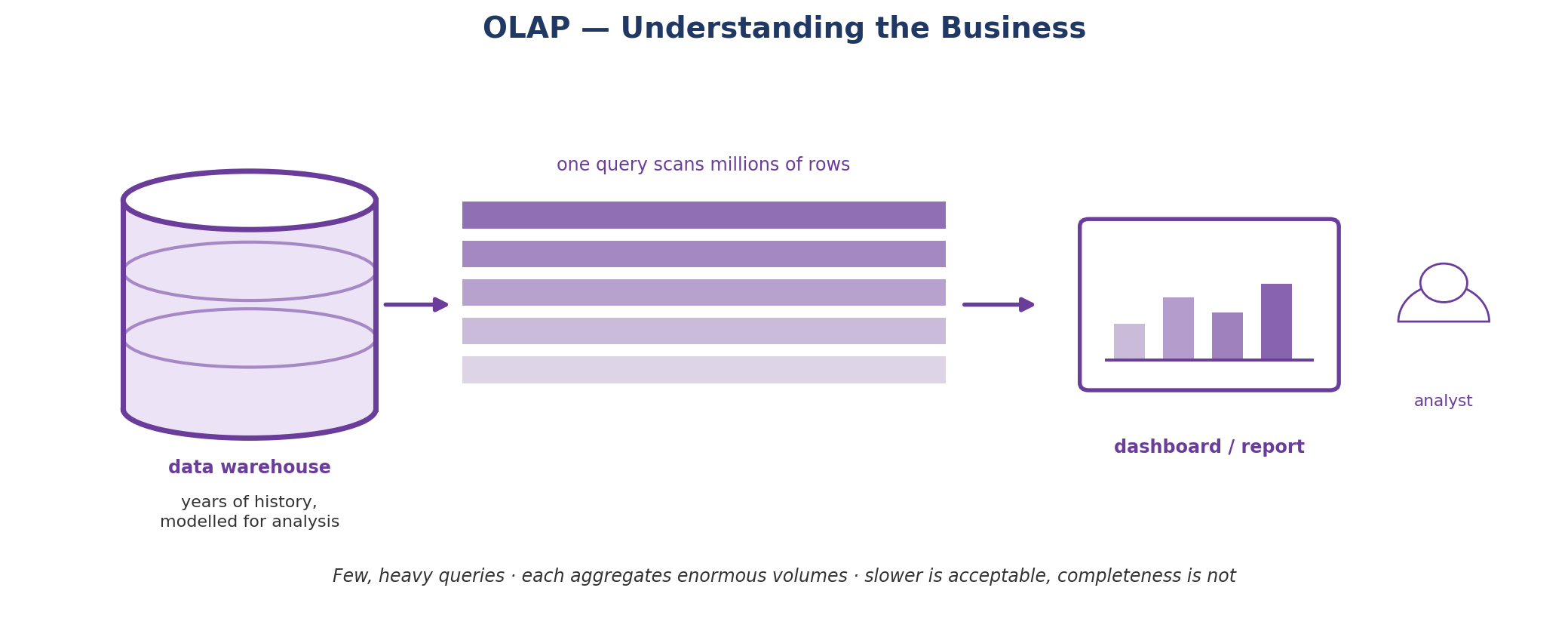
Figure 6.4 — An OLAP system answering an analytical question.

Characteristics

Workload: a small number of large, complex read queries; writes arrive in scheduled batches.
Rows touched: millions, aggregated down to a handful of output rows.
Priority: scan throughput and completeness; taking seconds or minutes is acceptable.
Data held: deep history, often denormalized into star or snowflake schemas for query speed.
Concurrency: comparatively few concurrent users — analysts and dashboards, not customers.
Storage layout: column-oriented, so a query reads only the fields it needs.

Typical systems: Snowflake, Google BigQuery, Amazon Redshift, SQL Server Analysis Services. Typical uses: BI dashboards, financial reporting, forecasting, cohort analysis.

6.7 OLTP vs. OLAP Compared

The two are not competing options — they are complementary systems tuned for opposite access patterns. Most organizations run both.

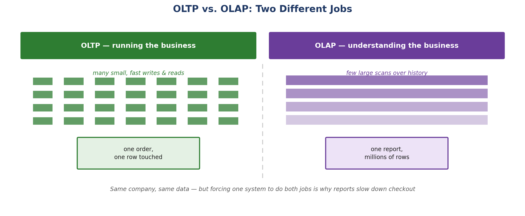
Figure 6.5 — Opposite workload shapes, side by side.

Aspect	OLTP	OLAP
Purpose	Record what is happening now	Explain what has happened
Query type	Simple, frequent, short	Complex, infrequent, long
Typical operation	Insert one order	Aggregate millions of rows
Rows per query	One to a few	Millions
Users	Thousands (customers, staff)	Tens (analysts, dashboards)
Data age	Current state	Deep history
Schema design	Normalized	Denormalized (star / snowflake)
Storage layout	Row-oriented	Column-oriented
Optimized for	Write speed, low latency	Scan throughput, aggregation
Response time	Milliseconds	Seconds to minutes
Examples	MySQL, PostgreSQL, Oracle	Snowflake, BigQuery, Redshift

6.8 Why the Storage Layout Differs

The performance gap between the two is not a matter of tuning — it comes from how bytes are physically arranged on disk.

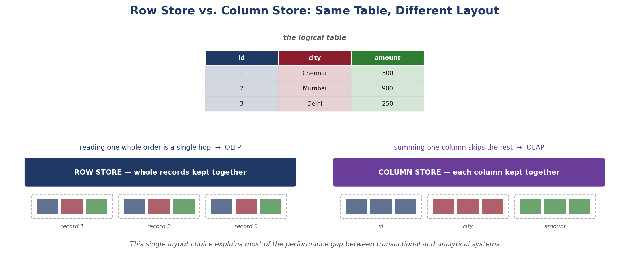
Figure 6.6 — Row-oriented versus column-oriented storage.

A row store keeps a full record contiguous, so fetching one order is a single read. A column store keeps each field contiguous, so summing one column never touches the others. Neither is better — they are tuned for opposite questions.

6.9 How the Two Worlds Connect

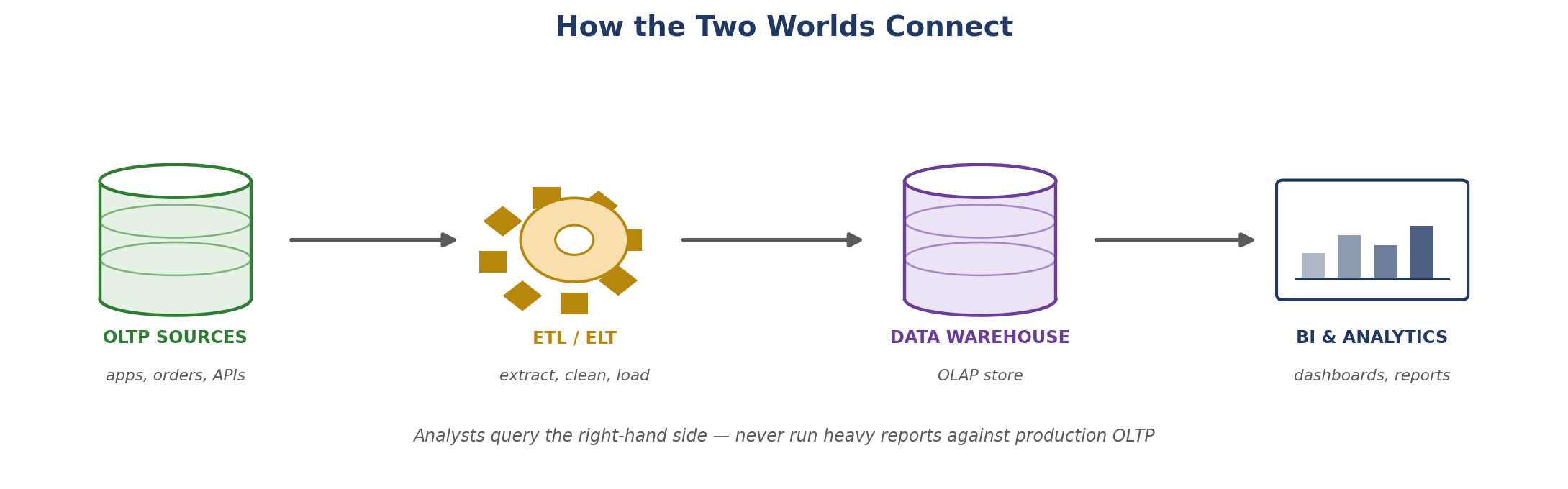
Figure 6.7 — From transactional sources to analytics.

Mature organizations run both: an OLTP database for operations and a separate OLAP warehouse for reporting, kept in sync by an ETL or ELT pipeline. Analysts query the right-hand side. Running heavy reports directly against production OLTP is the single most common cause of self-inflicted outages.

6.10 Choosing Deliberately

Shape of the data: naturally tabular, or nested and variable?
Workload: many small transactions, or few large scans?
Consistency needs: strict ACID, or is eventual consistency acceptable?
Scale: does this fit one server, or must it spread across many?
Operational appetite: self-managed, or a managed cloud service?

Best Practice: Select the database type from data structure, scale, transaction requirements, and reporting needs — not from what the team already knows.

Phase 2 – Relational Database Fundamentals

Phase 2 Overview

#	Subtopic	Learning Outcome
1	Relational Database Concepts	Schemas, tables, rows, columns, entities, attributes, records, data types, NULLs
2	Keys	Primary, foreign, candidate, alternate, super, composite, unique, natural, surrogate
3	Relationships	One-to-one, one-to-many, many-to-many, and parent-child tables
4	Database Design Basics	Entities, attributes, cardinality, ER diagrams, converting to tables
5	Normalization	Redundancy, anomalies, 1NF, 2NF, 3NF, BCNF, denormalization

Module 1: Relational Database Concepts

1.1 Database, Schema, Table

These three terms are often used loosely and mean different things. A database is the whole store. A schema is a named container inside it that groups related tables and defines their structure. A table holds the rows for one kind of thing.

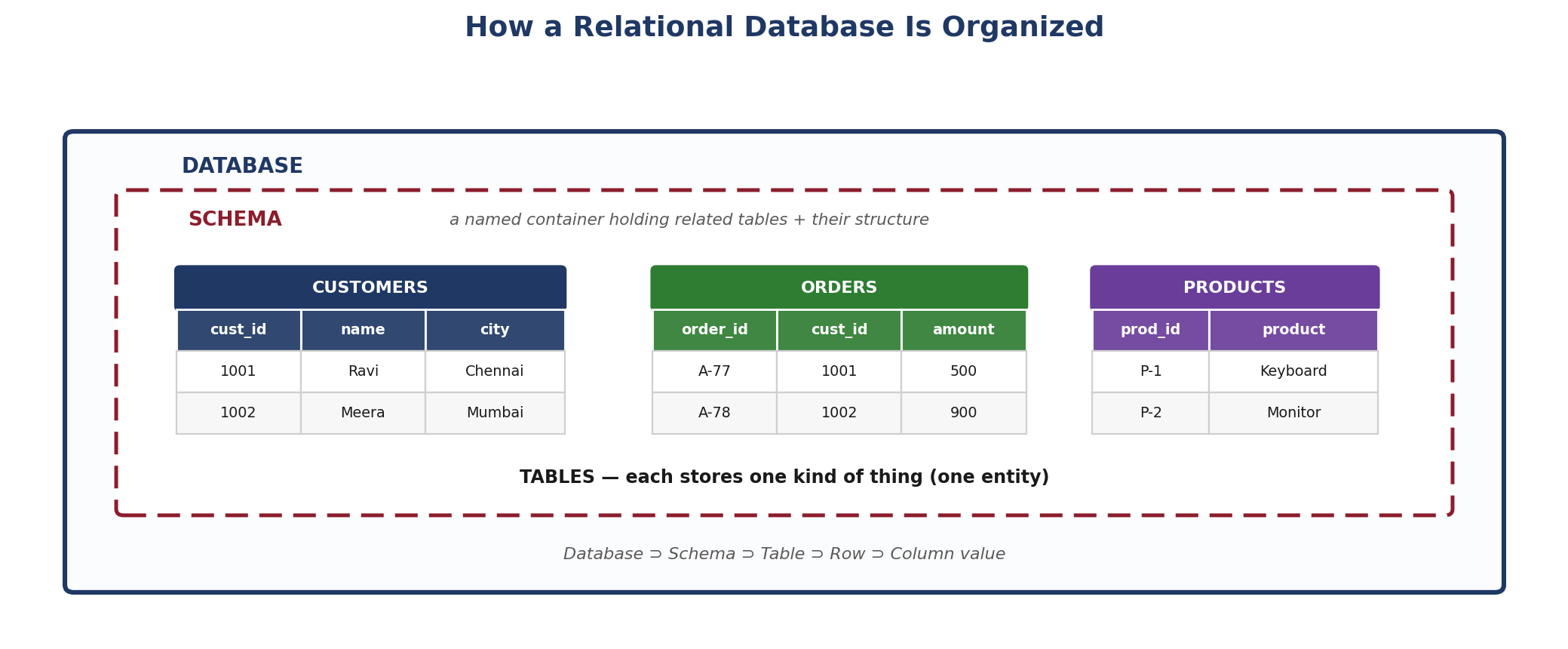
Figure 1.1 — Database contains schema contains table contains rows.

In PostgreSQL and SQL Server, a schema is an explicit object you create and grant permissions on. In MySQL, "schema" and "database" are effectively synonyms. The concept matters regardless of dialect: it is the unit at which structure and access are organized.

1.2 Entity, Attribute, Record

Design vocabulary and storage vocabulary describe the same things from different angles — knowing both prevents confusion when moving between an ER diagram and a live table.

Design term	Storage term	Meaning
Entity	Table	The real-world thing being stored — a customer, an order
Attribute	Column / field	One property of that thing — name, city, amount
Record / instance	Row / tuple	One specific occurrence — customer 1001
Attribute value	Cell	One value at the intersection of a row and column

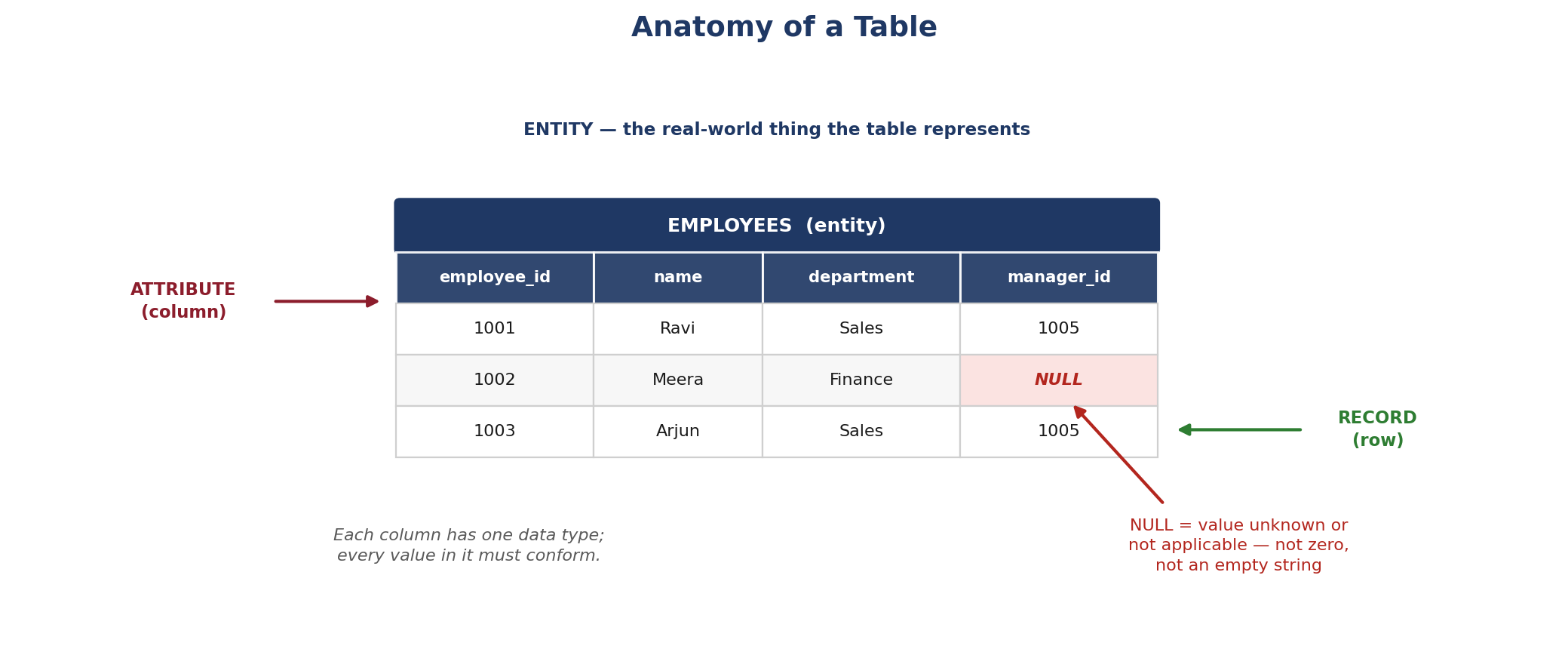
Figure 1.2 — The parts of a table, named.

1.3 Data Types

Every column is declared with a data type, and the database rejects any value that does not conform. This is the first and cheapest layer of data quality control — a text value can never end up in a numeric column by accident.

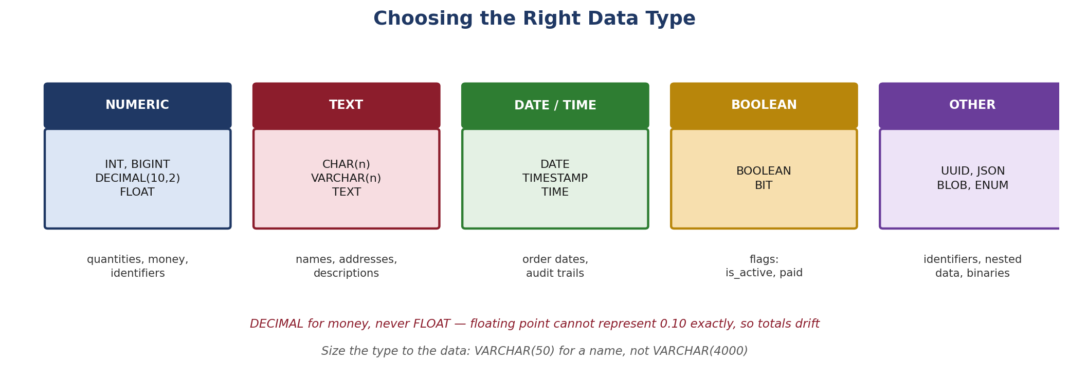
Figure 1.3 — The main data type families.

Use DECIMAL for money: FLOAT cannot represent 0.10 exactly, so repeated addition drifts. Financial totals must use exact decimal types.
Size to the data: VARCHAR(50) for a name rather than VARCHAR(4000) — oversized columns waste memory in sorts and joins.
Prefer native date types: storing dates as text prevents range queries, sorting, and date arithmetic.
Match key types exactly: a foreign key must share the parent's type; a mismatch silently disables index use on joins.

1.4 NULL Values

NULL means the value is unknown or not applicable. It is not zero, not an empty string, and not a blank space — it is the explicit absence of a value.

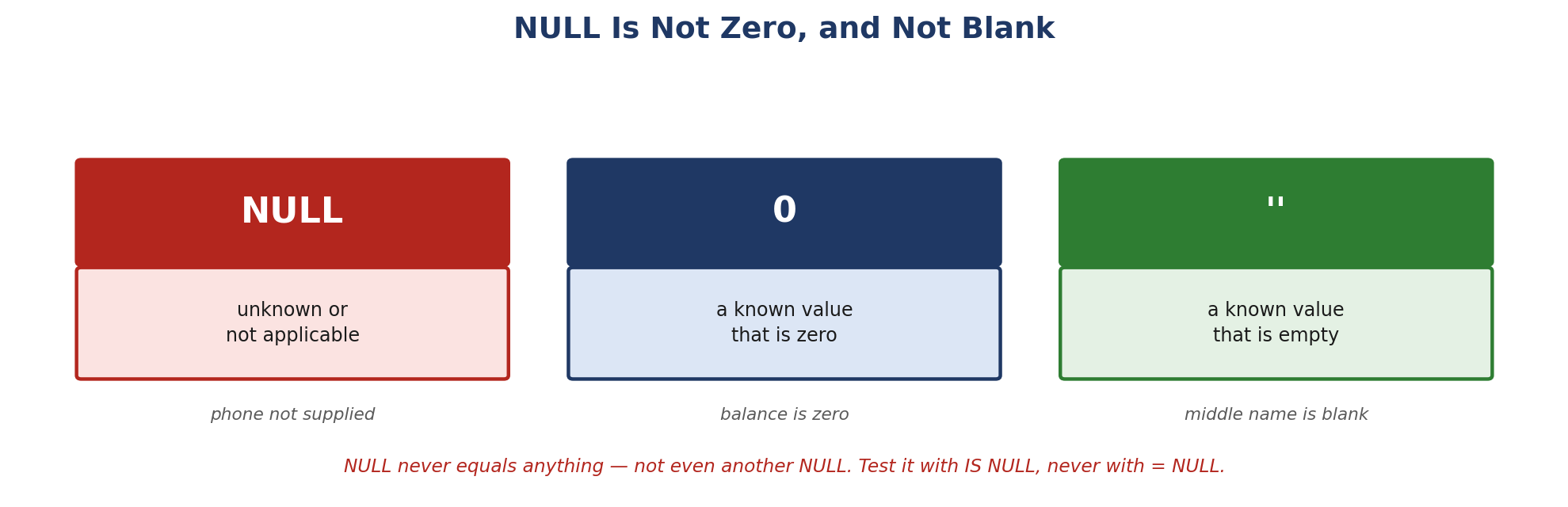
Figure 1.4 — Three different things that look similar.

Why NULL Behaves Unusually

Three-valued logic: comparisons involving NULL return UNKNOWN rather than TRUE or FALSE.
Equality fails: NULL = NULL is not true. Use IS NULL and IS NOT NULL instead.
Aggregates skip it: AVG and SUM ignore NULLs, so an average can be computed over fewer rows than expected.
Filters exclude it: WHERE city <> 'Chennai' will not return rows where city is NULL, which surprises most people the first time.
Primary keys forbid it: a primary key column can never be NULL.

Best Practice: Use meaningful table and column structures and appropriate data types.

Hands-On: Using a provided dataset, represent the data as relational tables and identify the schema, table, row, column, attribute, record, data type, and NULL values. For each column, state the data type you would declare and whether it should allow NULL.

Module 2: Keys

2.1 How the Key Types Nest

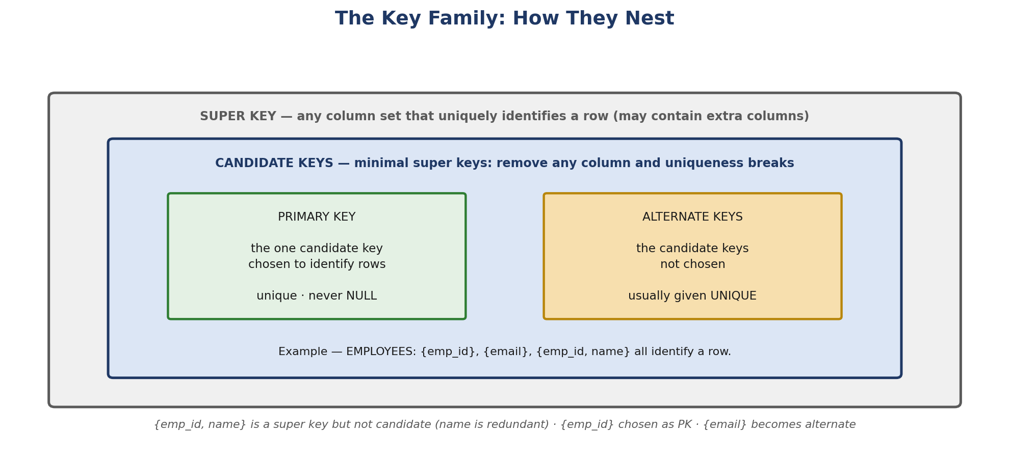
Figure 2.1 — Super key, candidate key, primary key, alternate key.

Super key: any set of columns that uniquely identifies a row — including sets with redundant extra columns.
Candidate key: a minimal super key. Remove any column from it and it stops being unique.
Primary key: the one candidate key chosen to identify rows. Unique, never NULL, and ideally never changing.
Alternate key: any candidate key not chosen as primary. Normally enforced with a UNIQUE constraint.

2.2 Primary Key and Foreign Key

These two do the structural work of the relational model. The primary key identifies a row within its table; the foreign key points from a child table to a parent row and makes the relationship enforceable.

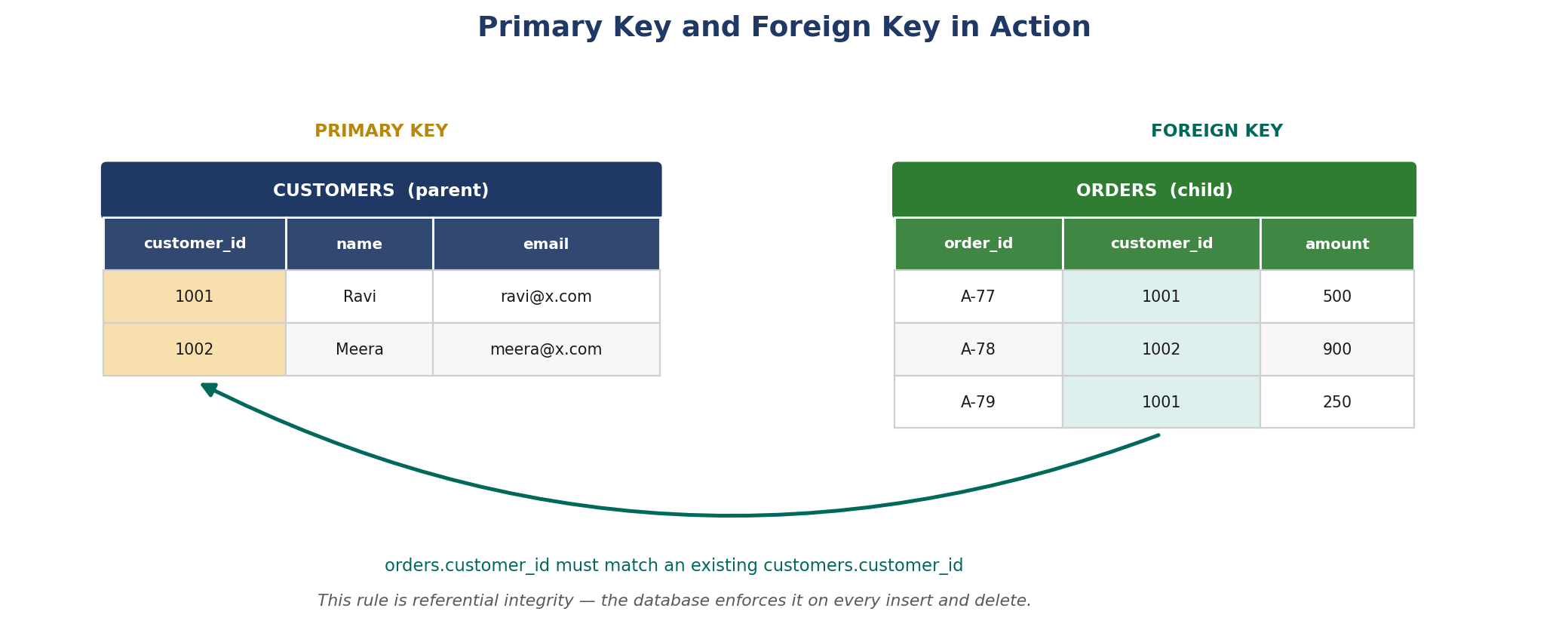
Figure 2.2 — A foreign key referencing a primary key.

Referential integrity means the database itself guarantees that every foreign key value matches a real parent row. An order cannot be inserted for a customer that does not exist, and deleting a customer with existing orders is either blocked or cascaded, according to the rule declared on the constraint.

2.3 Composite and Unique Keys

A composite key uses two or more columns together because no single column is unique on its own. This is the normal shape of a junction table's primary key.

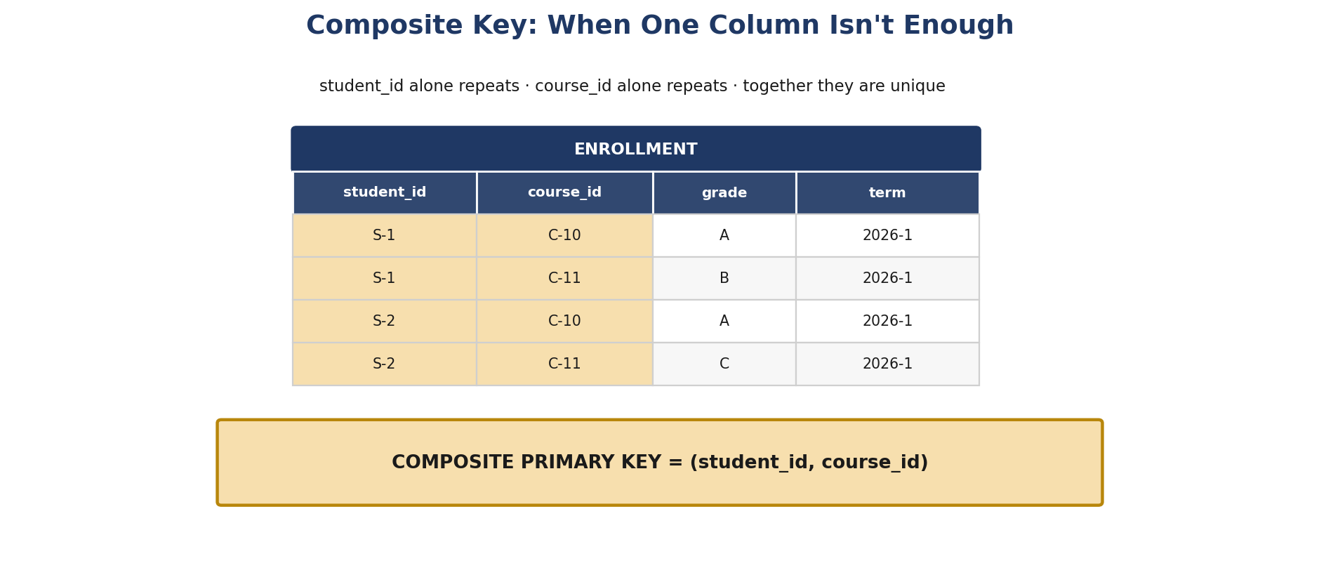
Figure 2.3 — A composite primary key across two columns.

A unique key enforces uniqueness on a column that is not the primary key — an email address, a national ID, a product SKU. Unlike a primary key, a unique key may allow a NULL (how many is dialect-dependent), and a table may have several.

2.4 Natural vs. Surrogate Keys

A natural key is a real business value that already identifies the row. A surrogate key is a meaningless value generated by the system purely to serve as an identifier.

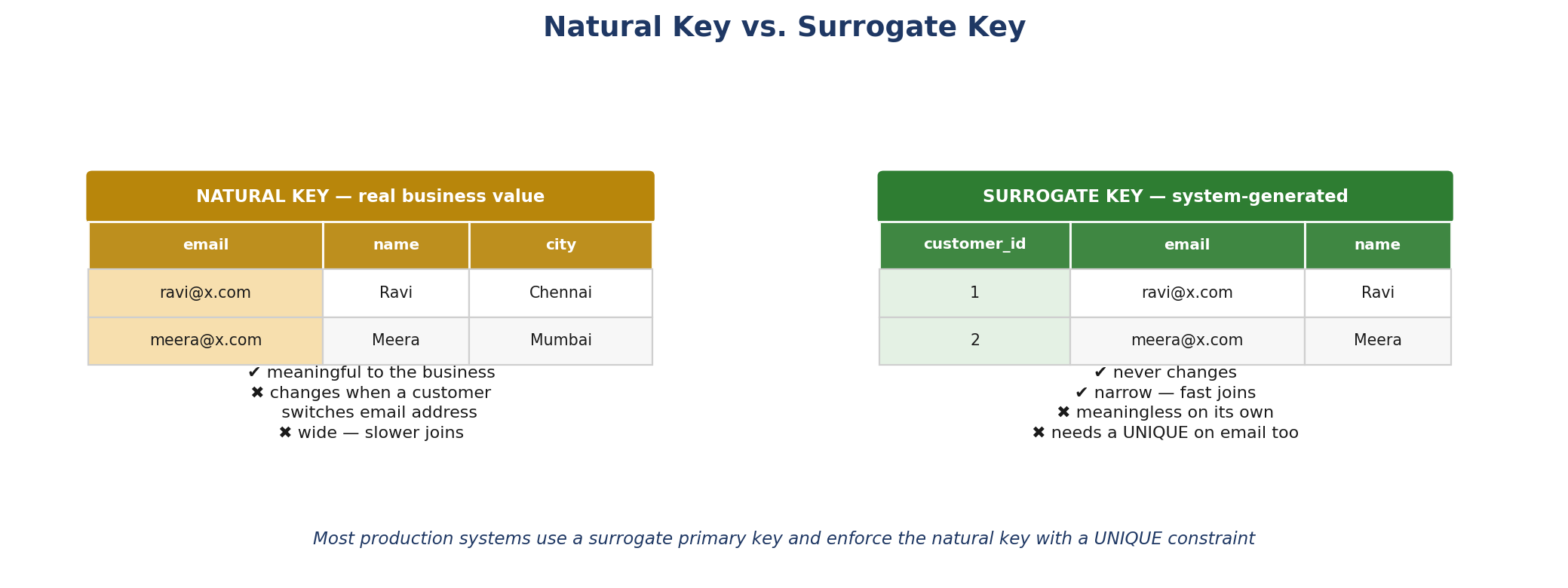
Figure 2.4 — The same table keyed two different ways.

	Natural Key	Surrogate Key
Source	Real business data	System-generated (sequence, identity, UUID)
Meaning	Meaningful on its own	None
Stability	Can change when the business changes	Never changes
Width	Often wide (text)	Narrow (integer)
Risk	A key change ripples to every child row	Duplicates possible unless natural key also constrained

Common practice is to use a surrogate primary key for stability and join performance, while still declaring a UNIQUE constraint on the natural key so genuine duplicates are impossible.

2.5 Summary of Key Types

Key	Definition	Example
Super	Any uniquely identifying column set	`{emp_id}`, `{emp_id, name}`
Candidate	Minimal super key	`{emp_id}`, `{email}`
Primary	The chosen candidate key	emp_id
Alternate	Candidate keys not chosen	email
Composite	Key spanning multiple columns	(student_id, course_id)
Unique	Enforces uniqueness, not the PK	email, national_id
Foreign	References another table's PK	orders.customer_id
Natural	Key drawn from business data	email, ISBN
Surrogate	System-generated identifier	customer_id 1, 2, 3

Best Practice: Primary keys should be stable, unique, and non-null.

Hands-On: Given four pre-defined tables and sample data, identify the Primary Key, Foreign Key, Candidate Key, Composite Key, Unique Key, Natural Key, and Surrogate Key where applicable. Where a table has more than one candidate key, state which you would choose as primary and why.

Module 3: Relationships

3.1 The Three Cardinalities

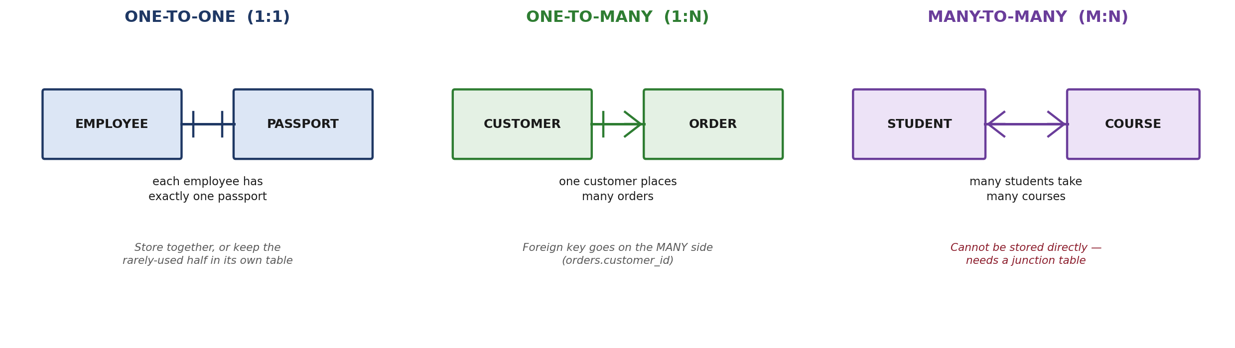
Figure 3.1 — One-to-one, one-to-many, and many-to-many.

One-to-One (1:1)

Each row in A relates to at most one row in B, and vice versa — an employee and their passport record. Genuine 1:1 relationships are uncommon; the data often belongs in a single table. Splitting is justified when one side is optional, rarely accessed, or has different security requirements. The foreign key goes on whichever side is optional, with a UNIQUE constraint to prevent it becoming 1:N.

One-to-Many (1:N)

One row in A relates to many rows in B, but each B row relates to only one A row — one customer, many orders. This is the most common relationship in practice. The foreign key always goes on the many side.

Many-to-Many (M:N)

Rows on both sides relate to many rows on the other — students and courses. This cannot be stored directly in two tables, because a foreign key column can only hold one value per row. It must be resolved with a third table.

3.2 Parent and Child Tables

In any foreign key relationship, the referenced table is the parent and the referencing table is the child. The child holds the foreign key; the parent knows nothing about it.

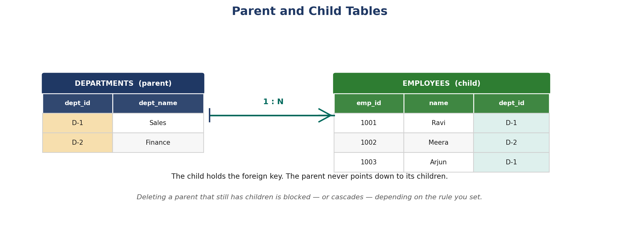
Figure 3.2 — The child table carries the foreign key.

Referential Actions

When a parent row is deleted or its key updated, the database applies the rule declared on the foreign key:

RESTRICT / NO ACTION: block the operation while children exist. The safe default.
CASCADE: delete or update the children automatically. Powerful and dangerous — a single delete can remove a great deal of data.
SET NULL: clear the child's foreign key, leaving the row orphaned but present.
SET DEFAULT: point the child at a predefined default parent row.

3.3 Resolving Many-to-Many

A junction table — also called a bridge, link, or associative table — sits between the two entities and holds a foreign key to each. The single M:N relationship becomes two 1:N relationships.

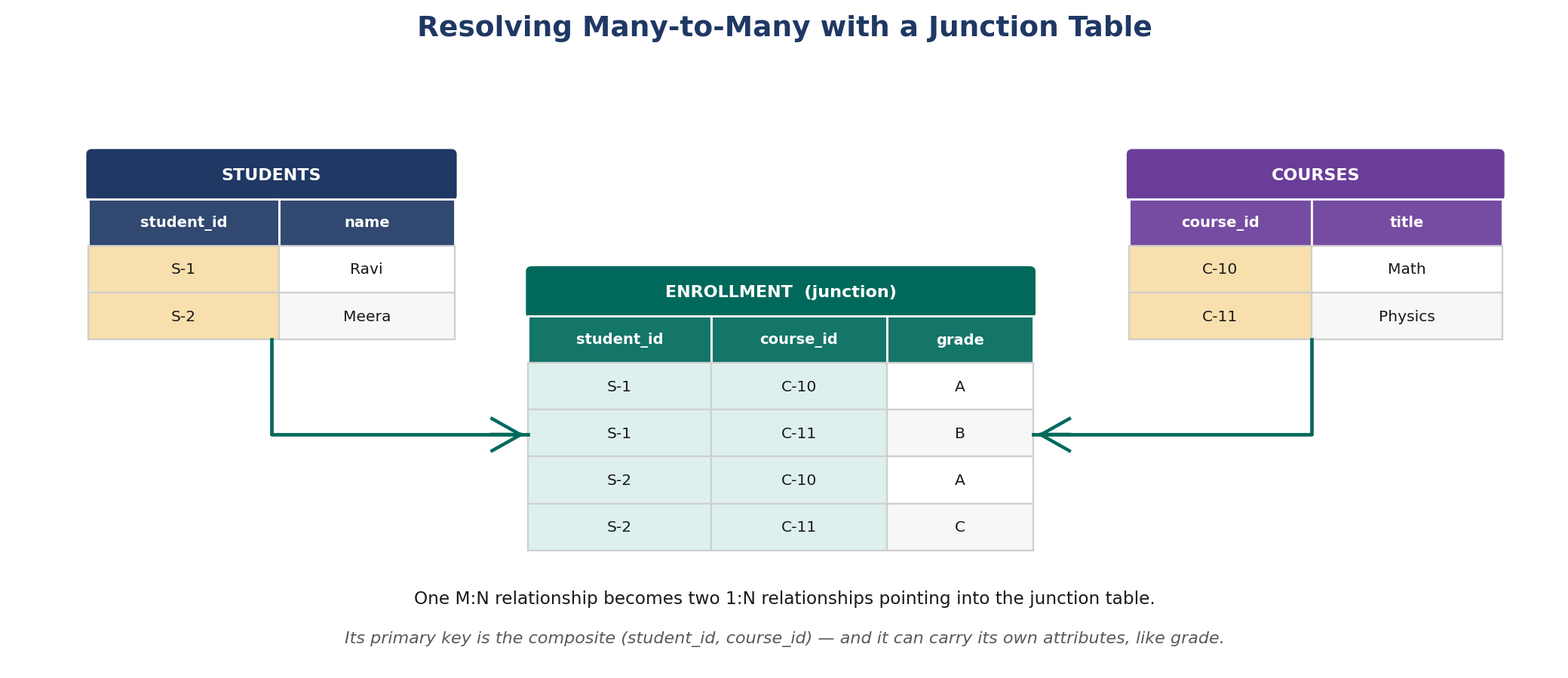
Resolving many-to-many with a junction table

Figure 3.3 — M:N resolved through a junction table.

Primary key: usually the composite of both foreign keys, which prevents duplicate pairings.
Own attributes: a junction table can carry data belonging to the relationship itself — a grade, an enrolment date, a quantity.
Naming: name it for what it represents (ENROLLMENT, ORDER_ITEM) rather than concatenating the two table names.

Best Practice: Define foreign keys wherever a relationship must be enforced, and use bridge tables for many-to-many relationships.

Hands-On: Given predefined tables and keys, identify the one-to-one, one-to-many, and many-to-many relationships, then create a junction table for the many-to-many case — defining its columns, its composite primary key, and both foreign keys.

Module 4: Database Design Basics

4.1 ER Diagram Notation

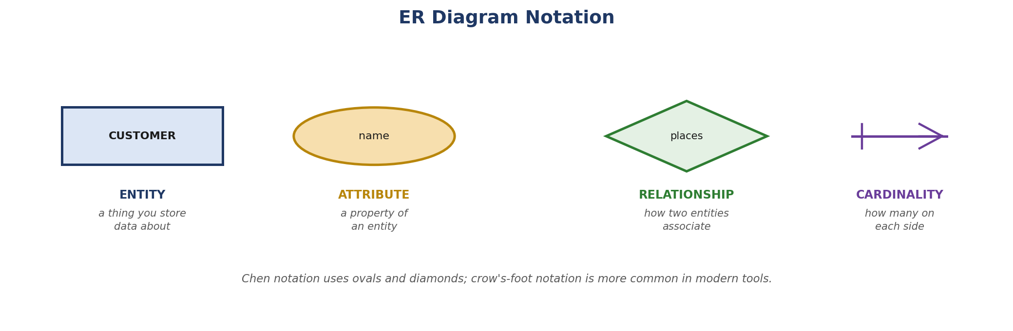
Figure 4.1 — The building blocks of an ER diagram.

Chen notation uses rectangles for entities, ovals for attributes, and diamonds for relationships. Crow's-foot notation — which lists attributes inside the entity box and shows cardinality with line endings — is more compact and is what most modern tools produce.

Reading Cardinality

A single bar: exactly one on that side.
A crow's foot: many on that side.
A circle: zero is allowed (optional).
Bar plus crow's foot: one or more — at least one is required.

4.2 From Requirements to Entities

A reliable first pass is grammatical: nouns in the requirement tend to become entities, verbs become relationships, and descriptive words become attributes.

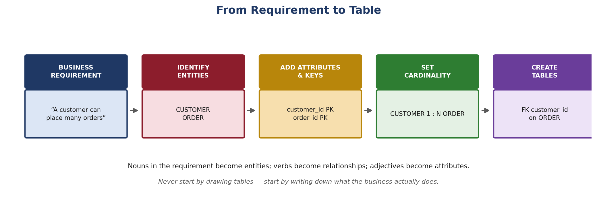
Figure 4.2 — The design sequence.

Gather requirements: understand what the business actually does before drawing anything.
Identify entities: the things that need to be stored and independently identified.
Identify attributes: what must be known about each entity, and which are mandatory.
Choose primary keys: natural or surrogate, one per entity.
Define relationships and cardinality: how entities associate, and how many on each side.
Convert to tables: apply the mapping rules and add foreign keys.
Normalize: check the result against the normal forms (Module 5).

4.3 A Worked ER Diagram

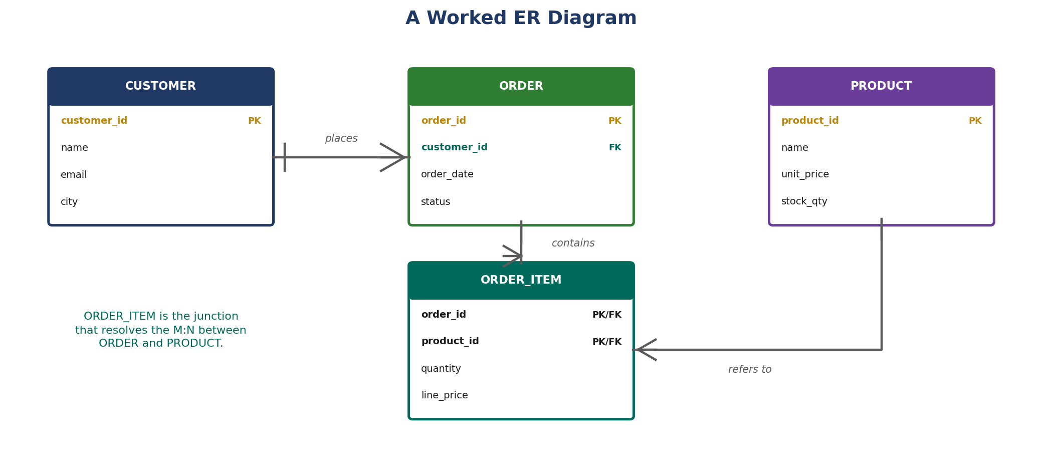
Figure 4.3 — A four-entity model with a resolved M:N relationship.

CUSTOMER to ORDER is one-to-many, so ORDER carries customer_id as a foreign key. ORDER to PRODUCT is many-to-many — an order contains many products and a product appears on many orders — so ORDER_ITEM resolves it, keyed on the pair (order_id, product_id) and carrying quantity and line price of its own.

4.4 Converting an ER Diagram to Tables

ER construct	Becomes	Rule
Entity	A table	One table per entity, named for the entity
Attribute	A column	With a data type and a NULL / NOT NULL decision
Primary key	PRIMARY KEY constraint	One per table, unique and non-null
1:1 relationship	FK on the optional side	Plus a UNIQUE constraint on that FK
1:N relationship	FK on the many side	The child references the parent's PK
M:N relationship	A junction table	Composite PK of both FKs
Multi-valued attribute	A separate table	One row per value, keyed back to the owner

Best Practice: Understand business requirements before creating tables.

Hands-On: Given an exact list of entities, attributes, primary keys, and relationships, draw an ER diagram and convert it into relational tables. Mark every primary key and foreign key, and state the cardinality of each relationship.

Module 5: Normalization

5.1 Redundancy and the Three Anomalies

When the same fact is stored in more than one place, the copies can disagree. Three specific failures follow, and they are the reason normalization exists.

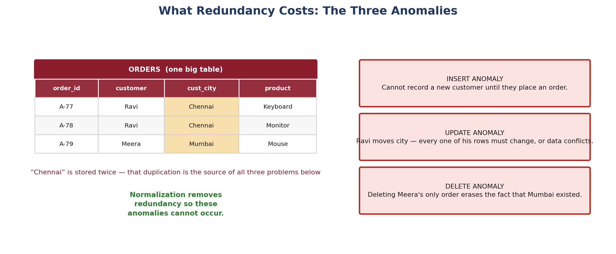
What redundancy costs: the three anomalies

Figure 5.1 — How redundancy produces anomalies.

Insert anomaly: a fact cannot be recorded because unrelated data is missing — a new customer cannot be added until they place an order.
Update anomaly: changing one fact requires updating many rows; miss one and the data now contradicts itself.
Delete anomaly: removing one fact destroys another — deleting a customer's only order also erases their city.

5.2 Functional Dependency

Normalization is defined in terms of functional dependency. Column B is functionally dependent on column A if each value of A determines exactly one value of B — written A → B. Knowing customer_id determines customer_city, so customer_id → customer_city.

The normal forms are simply rules about which dependencies are allowed to exist within one table.

5.3 First Normal Form (1NF)

A table is in 1NF when every cell holds a single atomic value, there are no repeating groups, and each column holds one kind of data.

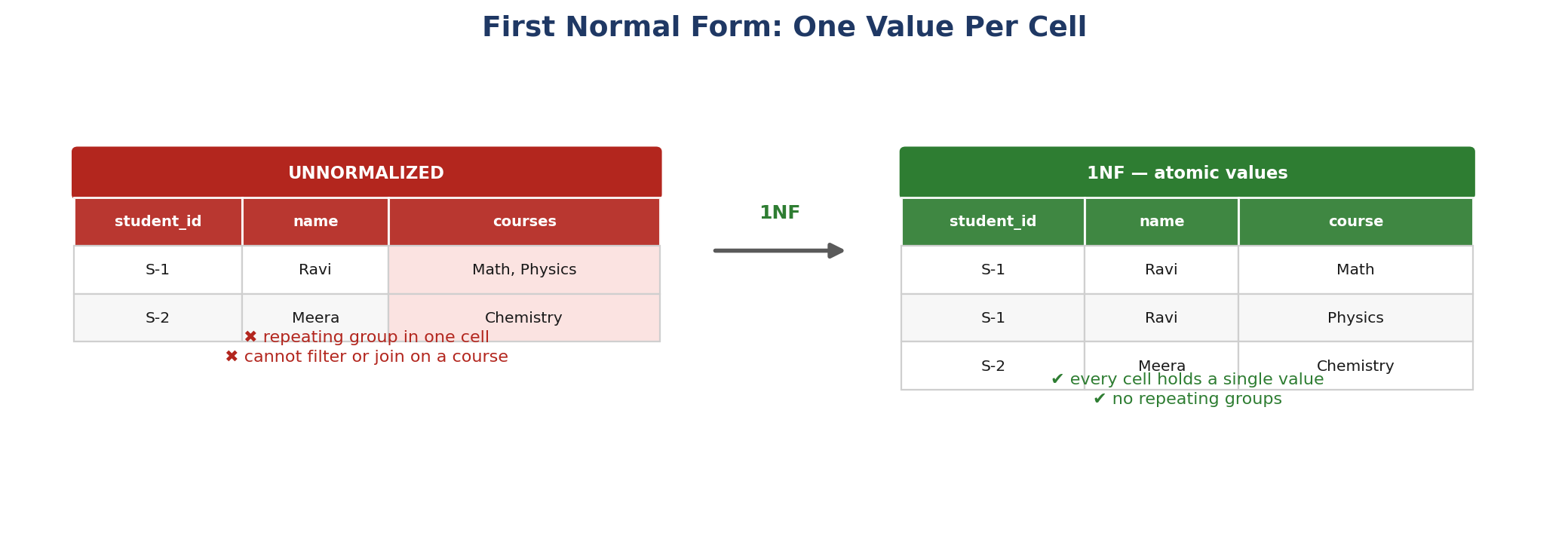
Figure 5.2 — Splitting a multi-valued cell into rows.

The common violation is a comma-separated list in one cell. It cannot be filtered, joined, or counted reliably, and any query against it degrades into string matching.

5.4 Second Normal Form (2NF)

A table is in 2NF when it is in 1NF and every non-key column depends on the whole primary key, not just part of it. This can only be violated when the primary key is composite.

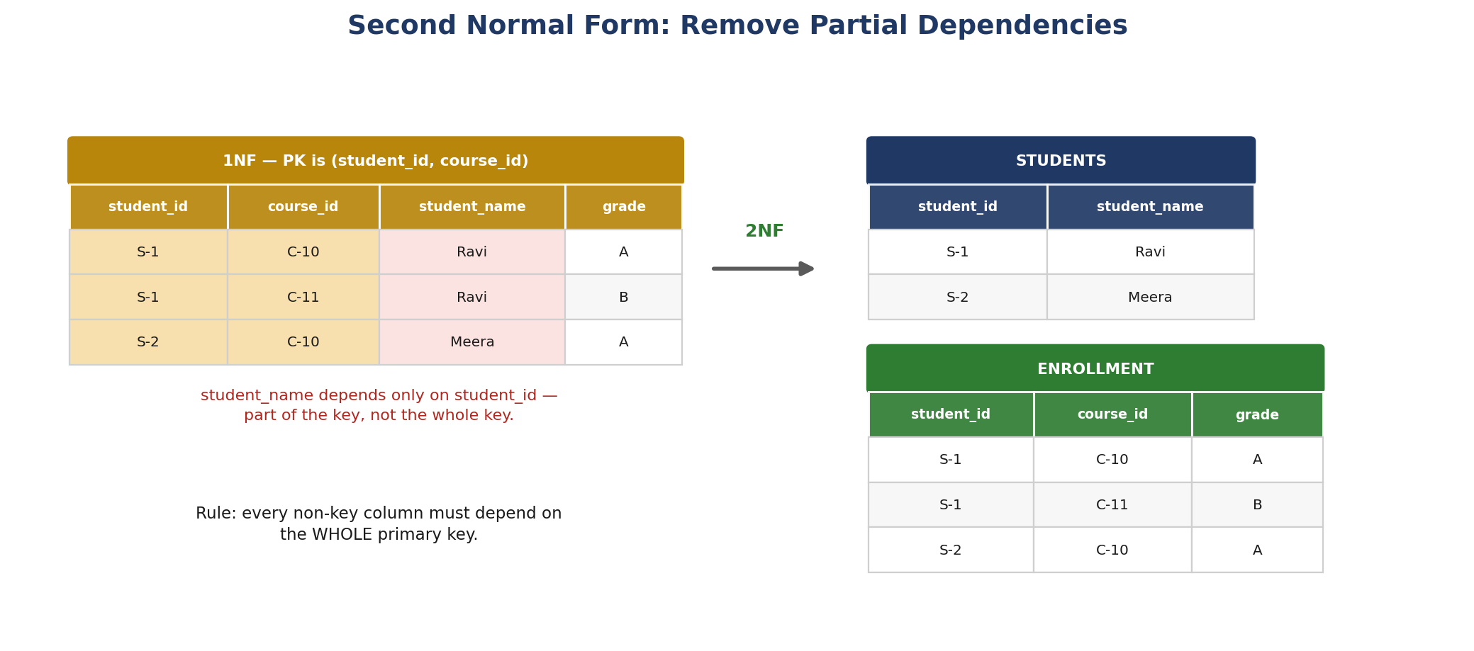
Second normal form: remove partial dependencies

Figure 5.3 — Removing a partial dependency.

In the example, the key is (student_id, course_id) but student_name depends on student_id alone. That is a partial dependency, and it causes the student's name to be repeated on every enrolment row. Moving it to a STUDENTS table stores it once.

5.5 Third Normal Form (3NF)

A table is in 3NF when it is in 2NF and no non-key column depends on another non-key column. Such an indirect chain is called a transitive dependency.

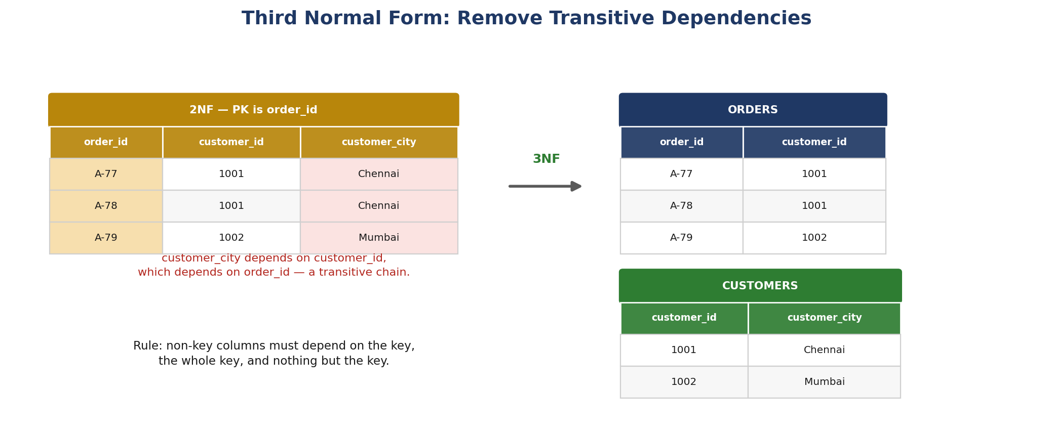
Third normal form: remove transitive dependencies

Figure 5.4 — Removing a transitive dependency.

The classic summary is that every non-key column must depend on the key, the whole key, and nothing but the key. 3NF is the practical target for most transactional systems.

5.6 Boyce-Codd Normal Form (BCNF)

BCNF is a stricter form of 3NF: for every functional dependency A → B, A must be a candidate key. A table can satisfy 3NF and still violate BCNF when it has overlapping candidate keys — for instance a scheduling table where (student, subject) determines a tutor, but each tutor teaches only one subject, so tutor → subject even though tutor is not a candidate key.

These situations are uncommon in ordinary business schemas, which is why 3NF is usually where normalization stops in practice.

5.7 The Normal Forms in Sequence

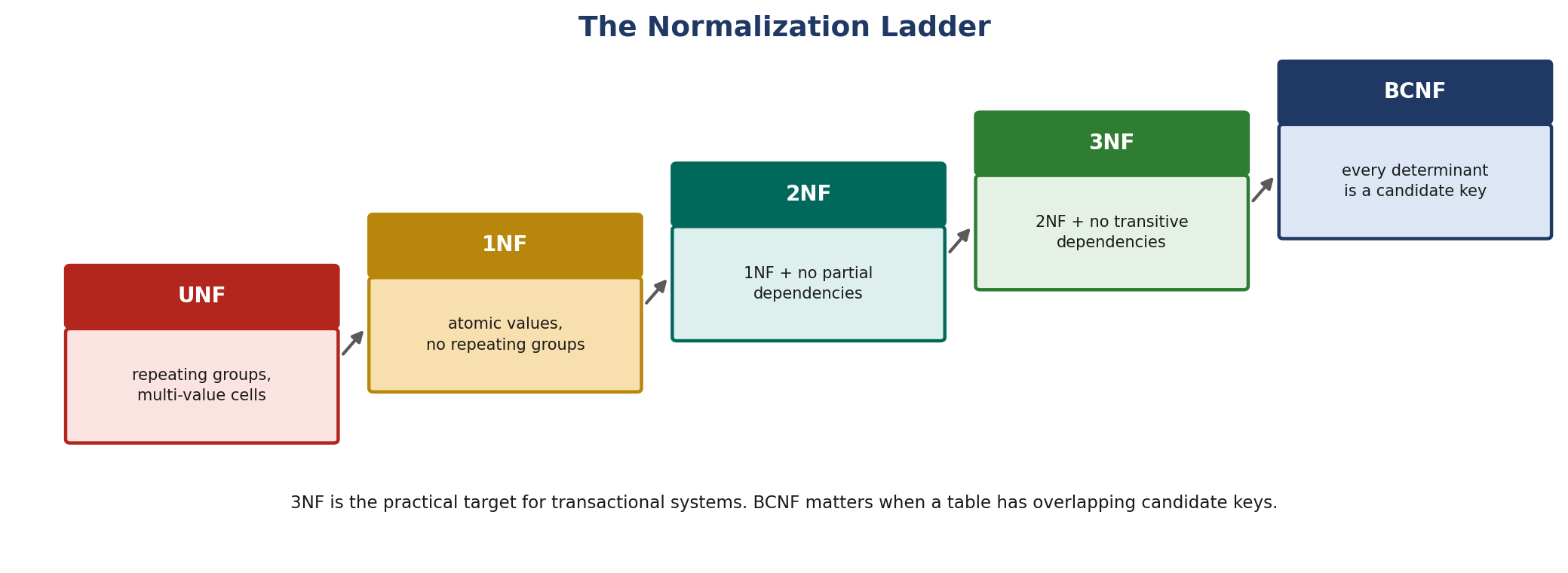
Figure 5.5 — Each form builds on the one before it.

Form	Requirement	Removes
1NF	Atomic values, no repeating groups	Multi-valued cells
2NF	1NF + no partial dependencies	Dependency on part of a composite key
3NF	2NF + no transitive dependencies	Non-key column depending on a non-key column
BCNF	Every determinant is a candidate key	Anomalies from overlapping candidate keys

5.8 Denormalization

Denormalization deliberately reintroduces redundancy to reduce the number of joins a query must perform. It is a considered trade-off, not a failure to normalize.

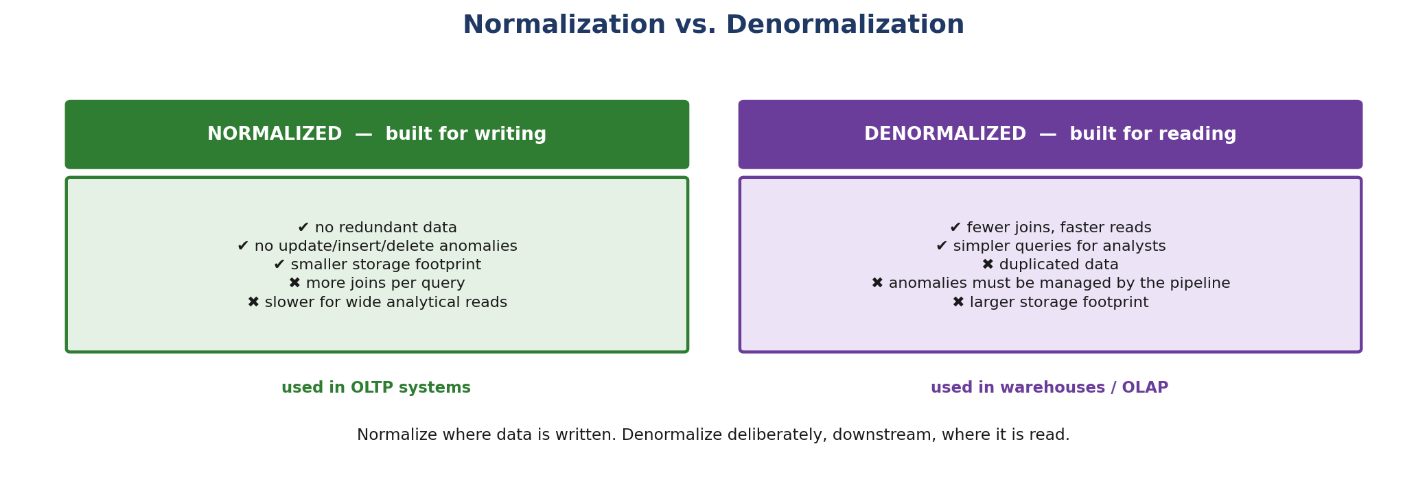
Figure 5.6 — Opposite optimizations for opposite workloads.

Where it belongs: reporting tables, data warehouses, and materialized views — the read-heavy side of the system.
Where it does not: the transactional tables that accept writes, where anomalies would corrupt the source of truth.
The obligation it creates: once data is duplicated, something must keep the copies in step — usually an ETL pipeline or a scheduled refresh.

Best Practice: Normalize transactional databases enough to eliminate redundancy — 3NF is the usual target — but avoid over-normalizing.

Phase 3 – SQL Fundamentals

Phase 3 Overview

Every concept is accompanied by runnable T-SQL. Scripts assume SQL Server and the SQL_Training_DB database created in Module 4.

#	Subtopic	Learning Outcome
1	Introduction to SQL	SQL purpose, ANSI SQL, dialects, SQL vs DBMS vs RDBMS
2	SQL Server Architecture	Protocol layer, SNI, TDS, relational engine, storage engine, buffer pool, files
3	Environment Setup & Configuration	Instances, services, authentication, connecting with SSMS
4	Creating & Managing Databases	CREATE, USE, inspect, ALTER, and safely DROP databases
5	Creating Database Objects – DDL	Schemas, tables, data types, ALTER, TRUNCATE, DROP
6	SQL Syntax Basics	Keywords, identifiers, literals, expressions, aliases, comments, formatting
7	SQL Naming Conventions	Naming standards for every object type
8	SQL Command Categories	DDL, DML, DQL, DCL, TCL and their impact
9	Basic Data Operations – DML	INSERT, UPDATE, DELETE performed safely
10	Basic SELECT – DQL	Column selection, aliases, expressions, DISTINCT

Module 1: Introduction to SQL

1.1 What Makes SQL Different

SQL is declarative. You state what result you want; the database decides how to produce it. A procedural language would require you to specify the loop, the index to use, and the join order. SQL requires none of that — the query optimizer makes those decisions.

-- You describe the result you want...
SELECT department, COUNT(*) AS employee_count
FROM   HR.Employees
WHERE  is_active = 1
GROUP  BY department;

-- ...you never write the loop, choose the index, or specify the join order.
-- The optimizer decides all of that at execution time.

Declarative intent: the same query may run a different way tomorrow if the data changes.

1.2 What SQL Is Used For

Defining structure: creating and altering databases, schemas, tables, and constraints.
Manipulating data: inserting, updating, and deleting rows.
Querying data: retrieving, filtering, joining, and aggregating — the bulk of an analyst's work.
Controlling access: granting and revoking permissions.
Managing transactions: grouping statements so they succeed or fail together.

1.3 SQL vs. DBMS vs. RDBMS

These three are routinely confused. They describe a language, a category of software, and a specific kind of that software.

Term	What it is	Example
SQL	A language — a syntax for expressing operations on relational data	`SELECT * FROM Employees;`
DBMS	Software that stores and manages data of any model	MongoDB, Redis, SQL Server
RDBMS	A DBMS that implements the relational model — tables, keys, constraints, and SQL	SQL Server, PostgreSQL, MySQL, Oracle

Put another way: every RDBMS is a DBMS, but not every DBMS is an RDBMS. SQL is the language most RDBMS products speak — it is not itself a database.

1.4 ANSI SQL and the Standard

SQL was standardized by ANSI in 1986 and by ISO in 1987, and has been revised repeatedly since — SQL-92 remains the most commonly cited baseline, with later revisions adding window functions (SQL:2003), JSON support (SQL:2016), and more.

No vendor implements the standard completely, and every vendor adds extensions. The practical consequence is that core SQL transfers everywhere, while convenience syntax often does not.

-- Standard SQL: runs unchanged on SQL Server, PostgreSQL, MySQL and Oracle
SELECT e.first_name,
       e.salary
FROM   Employees AS e
WHERE  e.salary > 50000
ORDER  BY e.salary DESC;

Core SELECT / FROM / WHERE / ORDER BY syntax is portable across every major RDBMS.

1.5 SQL Dialects

A dialect is a vendor's implementation of SQL plus its own extensions. The differences cluster in predictable places: row limiting, string handling, date functions, and procedural code.

Task	SQL Server (T-SQL)	PostgreSQL / MySQL	Oracle (PL/SQL)
Limit rows	`SELECT TOP 10 ...`	`... LIMIT 10`	`FETCH FIRST 10 ROWS ONLY`
Concatenate	`'a' + 'b'` or `CONCAT()`	`'a' \|\| 'b'`	`'a' \|\| 'b'`
Current date	`GETDATE()`	`NOW()` / `CURRENT_DATE`	`SYSDATE`
Null fallback	`ISNULL(col, 0)`	`COALESCE(col, 0)`	`NVL(col, 0)`

-- SQL Server (T-SQL)
SELECT TOP 10 employee_id, first_name + ' ' + last_name AS full_name
FROM   HR.Employees
ORDER  BY hire_date DESC;

-- PostgreSQL / MySQL equivalent
-- SELECT employee_id, first_name || ' ' || last_name AS full_name
-- FROM   employees
-- ORDER  BY hire_date DESC
-- LIMIT  10;

The same requirement, expressed two ways. COALESCE and CONCAT are the portable choices where available.

1.6 Why This Training Uses T-SQL

The remainder of this phase uses Microsoft SQL Server and its dialect, T-SQL, because that is the assigned training environment. Where a construct is vendor-specific rather than standard, it is flagged so the distinction stays visible.

Best Practice: Learn standard SQL first and treat vendor-specific syntax separately.

Module 2: SQL Server Architecture

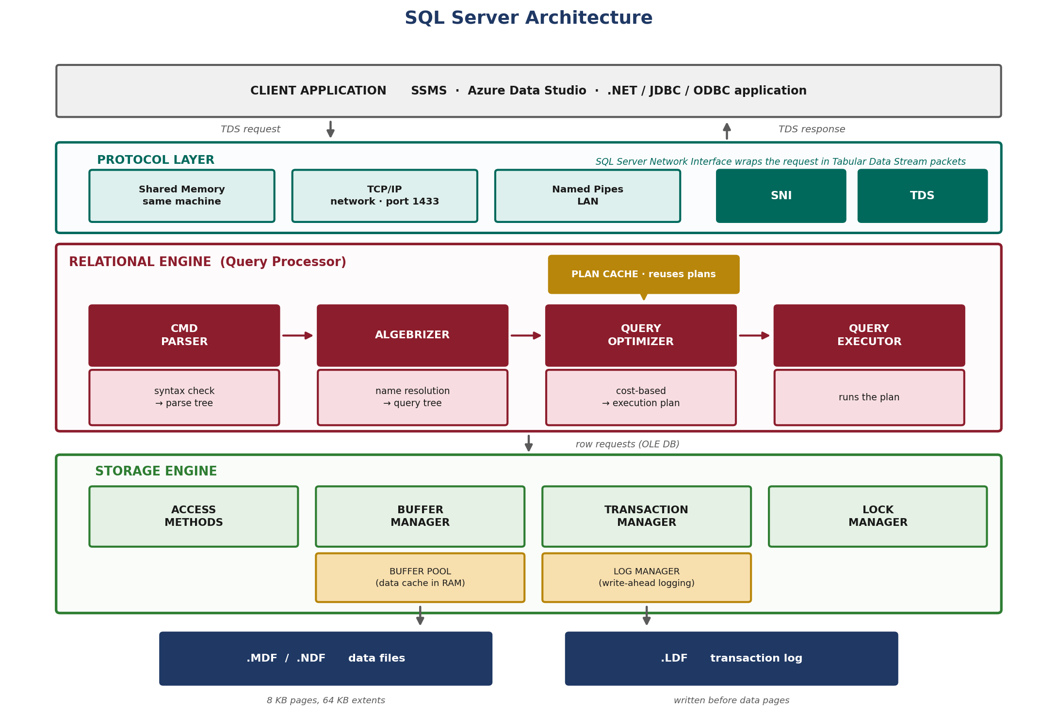
Figure 2.1 — The major components of a SQL Server instance.

2.1 Protocol Layer

The protocol layer accepts client connections and defines how bytes move between client and server. SQL Server supports three protocols:

Shared Memory: used when client and server are on the same machine. Fastest, no network stack involved, and the default for a local SSMS session.
TCP/IP: the standard for remote connections, listening on port 1433 by default for a default instance. Named instances use dynamic ports resolved through the SQL Server Browser service on UDP 1434.
Named Pipes: a LAN protocol using inter-process communication. Largely legacy, and often disabled.

SNI and TDS

SNI — the SQL Server Network Interface — is the protocol layer implementation shared by client and server. It wraps requests and results in TDS (Tabular Data Stream), the application-level protocol SQL Server speaks.

TDS is what carries your query text to the server and the result set back. Every driver — ODBC, JDBC, ADO.NET — ultimately produces TDS packets. When a connection is encrypted, TDS is wrapped in TLS at this layer.

-- Inspect how the current session is actually connected
SELECT session_id,
       net_transport,          -- TCP, Shared memory, Named pipe
       protocol_type,          -- TSQL
       encrypt_option,
       auth_scheme,            -- NTLM, KERBEROS, SQL
       local_tcp_port
FROM   sys.dm_exec_connections
WHERE  session_id = @@SPID;

sys.dm_exec_connections exposes the protocol layer for your own session.

2.2 Relational Engine (Query Processor)

The relational engine decides what to do. It never touches data files directly — it asks the storage engine for rows.

Command Parser

The parser checks syntax. If a keyword is misspelled or a bracket unclosed, the batch fails here and nothing else runs. On success it produces a parse tree. The parser also checks the plan cache first: if an identical statement already has a cached plan, the rest of compilation is skipped entirely.

Algebrizer (Binding)

The algebrizer resolves names and types. It verifies that every table, column, and function actually exists, that the user has the right to see them, and that data types are compatible. Its output is a query processor tree. This is the stage that produces "Invalid object name" errors — a syntactically perfect query referencing a non-existent table passes the parser and fails here.

Query Optimizer

The optimizer is cost-based. It generates candidate execution plans — different join orders, different index choices, different physical operators — estimates the cost of each using statistics about data distribution, and selects the cheapest it finds within its time budget.

It does not search exhaustively: for a complex query the plan space is enormous, so the optimizer stops once a plan is good enough.
It depends on statistics: stale statistics produce bad cardinality estimates, which produce bad plans. This is the single most common cause of sudden query slowdowns.
Its output is cached: plans are stored in the plan cache and reused for matching statements.

-- See the plan and the work a query actually does
SET STATISTICS IO, TIME ON;
GO

SELECT department, COUNT(*) AS headcount
FROM   HR.Employees
GROUP  BY department;
GO

SET STATISTICS IO, TIME OFF;
GO

-- In SSMS: Ctrl+M includes the actual execution plan with the results.
-- Ctrl+L shows the estimated plan without running the query.

STATISTICS IO reports logical reads — how many 8 KB pages the query touched.

Query Executor

The executor walks the chosen plan operator by operator, requesting rows from the storage engine through the OLE DB interface and assembling the result. It is also where runtime realities surface: a plan built for an estimated 10 rows that actually meets 10 million will still execute, just badly.

2.3 Storage Engine

The storage engine manages the physical reality — pages, files, memory, locks, and durability.

Access Methods

Access methods translate the executor's row requests into page requests, choosing between a table scan, an index seek, or an index scan, and handling the mechanics of reading and writing rows.

Buffer Manager and the Buffer Pool

The buffer pool is SQL Server's data cache in RAM. Every page read from disk is placed there first, and every page modified is modified there — never directly on disk.

Logical read: the page was found in the buffer pool. Fast.
Physical read: the page was not cached and had to come from disk. Orders of magnitude slower.
Dirty page: a page modified in memory but not yet written to disk.
Checkpoint: the process that flushes dirty pages to the data file, bounding recovery time after a crash.
Lazy writer: evicts least-recently-used pages when memory pressure demands it.

This is why running the same query twice is usually faster the second time: the first run paid for physical reads, the second was served from the buffer pool.

-- How much of the buffer pool is each database using?
SELECT DB_NAME(database_id)          AS database_name,
       COUNT(*) * 8 / 1024           AS cached_mb
FROM   sys.dm_os_buffer_descriptors
WHERE  database_id <> 32767          -- exclude the resource database
GROUP  BY DB_NAME(database_id)
ORDER  BY cached_mb DESC;

Each buffer descriptor represents one 8 KB page currently held in memory.

Transaction Manager and Write-Ahead Logging

The transaction manager guarantees the ACID properties. It works with the log manager under a rule called write-ahead logging (WAL): the log record describing a change must reach the transaction log on disk before the modified data page is allowed to be written.

That ordering is what makes both rollback and crash recovery possible. If the server fails, SQL Server replays the log — rolling forward committed transactions whose pages had not been written, and rolling back uncommitted ones.

Lock Manager

The lock manager provides isolation, coordinating shared and exclusive locks so concurrent sessions do not read or overwrite each other's uncommitted work. Blocking is this mechanism working as designed; a deadlock is two sessions each holding what the other needs, which SQL Server resolves by terminating one as the deadlock victim.

2.4 Physical Files

File	Extension	Purpose
Primary data file	.mdf	Startup information plus data; every database has exactly one
Secondary data file	.ndf	Optional additional data files, used to spread I/O
Transaction log	.ldf	Ordered record of every change; drives rollback and recovery

Data files are organized into 8 KB pages, the smallest unit SQL Server reads or writes. Eight contiguous pages form a 64 KB extent, the unit of space allocation. A row cannot span pages in the ordinary case, which is why an oversized row definition can fail even when the table is empty.

-- Physical files behind the current database
SELECT name                                   AS logical_name,
       type_desc,                             -- ROWS or LOG
       physical_name,
       size * 8 / 1024                        AS size_mb,
       CASE WHEN max_size = -1 THEN 'Unlimited'
            ELSE CAST(max_size * 8 / 1024 AS VARCHAR(20)) + ' MB'
       END                                    AS max_size,
       growth                                 AS growth_setting
FROM   sys.database_files;

size and max_size are stored as counts of 8 KB pages, hence the * 8 / 1024 conversion to MB.

2.5 The Full Journey of a Query

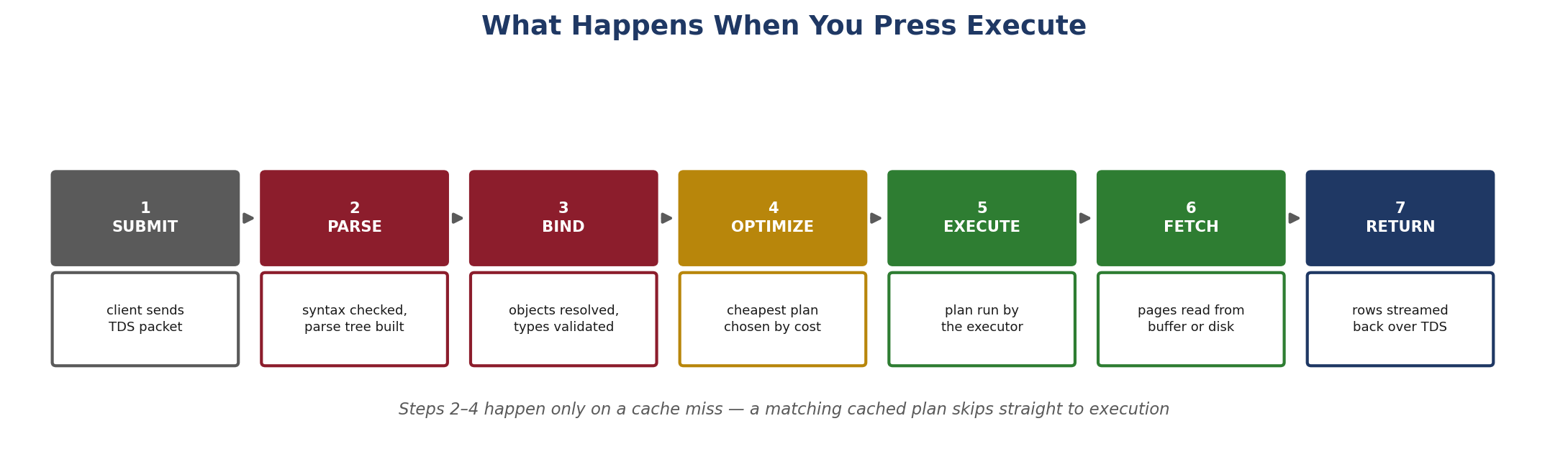
Figure 2.2 — Seven stages from Execute to result.

Best Practice: Understand the architecture conceptually before attempting performance tuning.

Module 3: SQL Server Environment Setup & Configuration

3.1 Editions

Edition	Cost	Typical use
Developer	Free	Full Enterprise feature set, licensed for development and testing only
Express	Free	Lightweight production use; capped at 10 GB per database
Standard	Licensed	Most production workloads
Enterprise	Licensed	Large scale, high availability, advanced features

Developer Edition is the correct choice for this training: it is free and functionally complete, so nothing in the course is blocked by a missing feature.

3.2 Instances

An instance is one running copy of the SQL Server engine, with its own service, its own memory, its own port, and its own set of databases. Multiple instances can coexist on one machine.

Default instance: referred to by the machine name alone, for example MYPC. Listens on TCP 1433.
Named instance: referred to as MACHINE\INSTANCENAME, for example MYPC\SQLEXPRESS. Uses a dynamic port discovered via the SQL Server Browser service.

A machine can host only one default instance but many named ones. Getting this wrong is the most frequent cause of a failed first connection.

3.3 Services

SQL Server runs as a set of Windows services. The engine service must be running before any connection can succeed.

Service	Purpose	Required?
SQL Server (MSSQLSERVER)	The database engine itself	Yes
SQL Server Agent	Scheduled jobs, alerts, maintenance plans	Only for scheduling
SQL Server Browser	Resolves named instances to their dynamic ports	For named instances
SQL Server Integration Services	ETL package execution	Only if using SSIS

Services are managed through SQL Server Configuration Manager, which is also where network protocols are enabled or disabled. Use it rather than the generic Windows Services console, because Configuration Manager applies the correct registry and permission changes.

3.4 Authentication Modes

SQL Server supports two ways of proving who you are, configured at the instance level.

	Windows Authentication	SQL Server Authentication
Credential source	Windows / Active Directory account	Login and password stored in SQL Server
Password handling	Managed by Windows; never sent by the app	Stored in master, supplied on connect
Policy enforcement	Domain policy applies automatically	Optional, via CHECK_POLICY
Best for	Domain-joined corporate environments	Cross-platform apps, non-domain clients
Security	Stronger — Kerberos/NTLM, no password in connection string	Weaker — credentials travel and are often hard-coded

"Mixed Mode" enables both. Windows Authentication is the recommended default; SQL Authentication should be enabled only when something genuinely cannot use a Windows identity.

-- Which authentication mode is this instance running?
SELECT SERVERPROPERTY('IsIntegratedSecurityOnly') AS windows_auth_only;
-- 1 = Windows Authentication only, 0 = Mixed Mode

-- How is the current session authenticated?
SELECT auth_scheme                       -- NTLM, KERBEROS or SQL
FROM   sys.dm_exec_connections
WHERE  session_id = @@SPID;

SERVERPROPERTY exposes instance-level configuration without opening the GUI.

3.5 Logins and Users

A login grants access to the instance. A user grants access to a specific database. The two are distinct objects, and a login with no mapped user can connect to the server but see nothing inside it.

-- Instance level: create a login
CREATE LOGIN training_user
WITH PASSWORD = 'StrongPassphrase!2026',
     CHECK_POLICY = ON;
GO

-- Database level: map that login to a user and grant rights
USE SQL_Training_DB;
GO

CREATE USER training_user FOR LOGIN training_user;
GO

ALTER ROLE db_datareader ADD MEMBER training_user;   -- read all tables
ALTER ROLE db_datawriter ADD MEMBER training_user;   -- insert/update/delete
GO

Grant the narrowest role that lets the person do their job — db_owner is rarely the right answer.

3.6 Connecting with SSMS

SQL Server Management Studio is the primary client. A connection needs four things:

Server name: MACHINE for a default instance, MACHINE\INSTANCE for a named one. localhost or a single dot both refer to the local default instance.
Authentication: Windows or SQL Server.
Credentials: supplied only for SQL Server authentication.
Encryption settings: newer SSMS versions default to encrypted connections; local training instances usually need Trust server certificate enabled.

-- Run these immediately after connecting to confirm where you are
SELECT @@SERVERNAME                       AS server_name;
SELECT @@VERSION                          AS version_details;
SELECT SERVERPROPERTY('MachineName')      AS machine_name,
       SERVERPROPERTY('InstanceName')     AS instance_name,
       SERVERPROPERTY('Edition')          AS edition,
       SERVERPROPERTY('ProductVersion')   AS product_version,
       SERVERPROPERTY('ProductLevel')     AS service_pack_level;

SELECT DB_NAME()                          AS current_database;
SELECT SUSER_NAME()                       AS login_name,
       USER_NAME()                        AS database_user_name;

A NULL instance_name means you are connected to the default instance.

When a Connection Fails

Symptom	Usual cause
Network-related or instance-specific error	Engine service not running, or wrong instance name
Login failed for user (Error 18456)	Wrong password, or SQL Authentication not enabled
Cannot connect to a named instance remotely	SQL Server Browser stopped, or UDP 1434 blocked
Timeout expired	TCP/IP protocol disabled, or port 1433 blocked by firewall
Certificate chain error	Encryption required without Trust server certificate

Best Practice: Use development and training environments for practice, apply appropriate authentication, and never expose privileged credentials.

Hands-On: Install or set up the assigned SQL Server environment. Identify the server and instance name, start and verify the SQL Server service in Configuration Manager, open SSMS, and connect successfully. Confirm the connection by running the verification script in section 3.6 and recording the server name, edition, and authentication scheme.

Module 4: Creating & Managing Databases

4.1 Instance vs. Database

	Instance (server)	Database
What it is	A running copy of the engine	A container of tables and other objects
Identified by	MACHINE\INSTANCE	A name unique within the instance
Security object	Login	User
Contains	Many databases	Schemas, tables, views, procedures
Its own files	No — shared binaries	Yes — .mdf and .ldf

4.2 System Databases

Every instance ships with four system databases. They are not for user data, and understanding what they do prevents costly mistakes.

master: instance-wide metadata — logins, linked servers, configuration. If master is lost, the instance will not start.
model: the template for every new database. Objects added here appear in all databases created afterwards.
msdb: SQL Server Agent jobs, schedules, alerts, and backup history.
tempdb: temporary tables, table variables, sort and hash spills. Recreated from scratch every time the service restarts.

4.3 Creating a Database

-- Simplest form: everything inherited from the model database
CREATE DATABASE SQL_Training_DB;
GO

Adequate for training; file locations and sizes come from the model database defaults.

Production databases are normally created with explicit file definitions, because sizing files up front avoids repeated autogrowth events that fragment storage and pause the workload.

-- Explicit form: control file names, locations, sizes and growth
CREATE DATABASE SQL_Training_DB
ON PRIMARY
(
    NAME       = N'SQL_Training_DB_Data',
    FILENAME   = N'C:\SQLData\SQL_Training_DB.mdf',
    SIZE       = 256MB,
    MAXSIZE    = 4096MB,
    FILEGROWTH = 128MB            -- fixed size, not a percentage
)
LOG ON
(
    NAME       = N'SQL_Training_DB_Log',
    FILENAME   = N'C:\SQLLogs\SQL_Training_DB.ldf',
    SIZE       = 128MB,
    MAXSIZE    = 2048MB,
    FILEGROWTH = 64MB
);
GO

Prefer a fixed FILEGROWTH in MB over a percentage — percentage growth accelerates as the file gets larger.

4.4 Selecting and Inspecting a Database

USE changes the session's current database context. Every unqualified object name is resolved against whatever database is current — which is why running a script in the wrong context is such a common and damaging error.

USE SQL_Training_DB;
GO

SELECT DB_NAME() AS current_database;       -- always confirm before running DDL/DML

-- List every database on this instance
SELECT database_id,
       name,
       create_date,
       state_desc,                          -- ONLINE, OFFLINE, RESTORING
       recovery_model_desc,                 -- FULL, SIMPLE, BULK_LOGGED
       collation_name
FROM   sys.databases
ORDER  BY name;

-- Size and growth of the current database's files
SELECT name           AS logical_name,
       type_desc,
       physical_name,
       size * 8 / 1024 AS size_mb
FROM   sys.database_files;

-- Does a specific database exist?
IF DB_ID('SQL_Training_DB') IS NOT NULL
    PRINT 'SQL_Training_DB exists.';
ELSE
    PRINT 'SQL_Training_DB not found.';

DB_NAME() is the cheapest habit in SQL Server — run it before anything destructive.

4.5 Altering a Database

-- Rename a database
ALTER DATABASE SQL_Training_DB MODIFY NAME = SQL_Training_DB_2026;
GO

-- Change the recovery model
-- SIMPLE: log truncates automatically, no point-in-time restore
-- FULL:   every change retained until a log backup, enables point-in-time restore
ALTER DATABASE SQL_Training_DB SET RECOVERY SIMPLE;
GO

-- Grow the data file
ALTER DATABASE SQL_Training_DB
MODIFY FILE (NAME = N'SQL_Training_DB_Data', SIZE = 512MB);
GO

-- Force single-user mode, disconnecting others (needed before some operations)
ALTER DATABASE SQL_Training_DB
SET SINGLE_USER WITH ROLLBACK IMMEDIATE;
GO

-- Return to normal
ALTER DATABASE SQL_Training_DB SET MULTI_USER;
GO

ROLLBACK IMMEDIATE terminates other sessions and rolls back their open transactions — never run it casually on a shared server.

4.6 Dropping a Database

DROP DATABASE deletes the database and its files from disk. There is no recycle bin and no undo. The only recovery path is a restore from backup, which assumes a backup exists.

-- Safe drop pattern: verify context, confirm the target, then drop
USE master;                                  -- cannot drop the database you are in
GO

-- Step 1: confirm exactly what will be removed
SELECT name, database_id, create_date
FROM   sys.databases
WHERE  name = 'SQL_Test_DB';

-- Step 2: check nobody else is connected
SELECT session_id, login_name, host_name, status
FROM   sys.dm_exec_sessions
WHERE  database_id = DB_ID('SQL_Test_DB');

-- Step 3: drop only if it exists, and only the intended target
IF DB_ID('SQL_Test_DB') IS NOT NULL
BEGIN
    ALTER DATABASE SQL_Test_DB SET SINGLE_USER WITH ROLLBACK IMMEDIATE;
    DROP DATABASE SQL_Test_DB;
    PRINT 'SQL_Test_DB dropped.';
END
ELSE
    PRINT 'SQL_Test_DB does not exist - nothing dropped.';
GO

The IF DB_ID(...) IS NOT NULL guard makes the script safe to run more than once.

Best Practice: Use meaningful database names, and never DROP a database without verifying the target and confirming it is safe.

Hands-On: Create SQL_Training_DB and verify it appears in SSMS Object Explorer. Switch to it with USE and confirm with DB_NAME(). Inspect its properties through sys.databases and sys.database_files. Create a second database named SQL_Test_DB, then safely drop only SQL_Test_DB using the guarded pattern in section 4.6 — confirming afterwards that SQL_Training_DB is untouched.

Module 5: Creating Database Objects – DDL

One property separates DDL from everything else: in SQL Server, DDL statements auto-commit. Unless you explicitly wrap them in a transaction, they take effect immediately and cannot be undone.

5.1 Schemas

A schema is a namespace inside a database. It groups related objects, simplifies permission management — rights can be granted on the whole schema at once — and prevents name collisions. Every object belongs to exactly one schema; if none is specified, dbo is used.

USE SQL_Training_DB;
GO

CREATE SCHEMA HR AUTHORIZATION dbo;
GO

CREATE SCHEMA Sales AUTHORIZATION dbo;
GO

-- List the schemas in this database
SELECT s.name AS schema_name,
       p.name AS owner_name
FROM   sys.schemas AS s
JOIN   sys.database_principals AS p ON s.principal_id = p.principal_id
WHERE  s.name NOT IN ('sys', 'INFORMATION_SCHEMA')
ORDER  BY s.name;

-- Permissions can then be granted once, for everything in the schema
GRANT SELECT ON SCHEMA::HR TO training_user;
GO

CREATE SCHEMA must be the first statement in its batch, hence the GO separators.

5.2 Data Types

Every column is declared with a data type. Choosing correctly affects storage, performance, and correctness.

Category	Types	Notes
Exact numeric	TINYINT, SMALLINT, INT, BIGINT, DECIMAL(p,s), NUMERIC, MONEY	INT covers ±2.1 billion; use DECIMAL for money
Approximate numeric	FLOAT, REAL	Binary floating point — never use for currency
Character	CHAR(n), VARCHAR(n), VARCHAR(MAX)	Fixed vs variable length; MAX allows up to 2 GB
Unicode character	NCHAR(n), NVARCHAR(n), NVARCHAR(MAX)	Two bytes per character; required for multi-language text
Date and time	DATE, TIME, DATETIME2(n), DATETIMEOFFSET, SMALLDATETIME	Prefer DATETIME2 over the legacy DATETIME
Other	BIT, UNIQUEIDENTIFIER, VARBINARY(MAX), XML	BIT stores 0, 1 or NULL

Choosing Between Similar Types

CHAR vs VARCHAR: CHAR(10) always occupies 10 characters, padding with spaces; VARCHAR(10) stores only what is supplied plus 2 bytes of overhead. Use CHAR only for genuinely fixed-length codes such as a country code.
VARCHAR vs NVARCHAR: NVARCHAR supports any language but costs double the bytes. Use it when names, addresses, or free text may be non-Latin.
DECIMAL vs FLOAT: DECIMAL(10,2) is exact; FLOAT is not. Money, quantities, and anything summed must be DECIMAL.
DATETIME vs DATETIME2: DATETIME2 has a wider range, better precision, and standard behaviour. DATETIME is retained only for legacy compatibility.
Sizing: declare the size you need. VARCHAR without a length defaults to 1 character in some contexts and 30 in others — always be explicit.

5.3 Creating Tables

USE SQL_Training_DB;
GO

-- Parent table: departments
CREATE TABLE HR.Departments
(
    DepartmentID    INT            NOT NULL IDENTITY(1,1),
    DepartmentName  NVARCHAR(100)  NOT NULL,
    Location        NVARCHAR(100)  NULL,
    CreatedDate     DATETIME2(0)   NOT NULL
        CONSTRAINT DF_Departments_CreatedDate DEFAULT (SYSDATETIME()),

    CONSTRAINT PK_Departments PRIMARY KEY CLUSTERED (DepartmentID),
    CONSTRAINT UQ_Departments_Name UNIQUE (DepartmentName)
);
GO

-- Child table: employees
CREATE TABLE HR.Employees
(
    EmployeeID      INT            NOT NULL IDENTITY(1001,1),
    FirstName       NVARCHAR(50)   NOT NULL,
    LastName        NVARCHAR(50)   NOT NULL,
    Email           NVARCHAR(150)  NULL,
    HireDate        DATE           NOT NULL,
    Salary          DECIMAL(10,2)  NOT NULL,
    DepartmentID    INT            NULL,
    ManagerID       INT            NULL,
    IsActive        BIT            NOT NULL
        CONSTRAINT DF_Employees_IsActive DEFAULT (1),

    CONSTRAINT PK_Employees PRIMARY KEY CLUSTERED (EmployeeID),
    CONSTRAINT UQ_Employees_Email UNIQUE (Email),
    CONSTRAINT CK_Employees_Salary CHECK (Salary > 0),
    CONSTRAINT FK_Employees_Departments FOREIGN KEY (DepartmentID)
        REFERENCES HR.Departments (DepartmentID),
    CONSTRAINT FK_Employees_Manager FOREIGN KEY (ManagerID)
        REFERENCES HR.Employees (EmployeeID)
);
GO

Naming every constraint explicitly means error messages identify the rule that was violated.

Note the self-referencing foreign key on ManagerID: a manager is also an employee, so the table points at itself. This is how hierarchies are modelled in a single table.

-- Projects, and the junction table resolving the M:N with employees
CREATE TABLE HR.Projects
(
    ProjectID       INT            NOT NULL IDENTITY(1,1),
    ProjectName     NVARCHAR(150)  NOT NULL,
    StartDate       DATE           NOT NULL,
    EndDate         DATE           NULL,
    Budget          DECIMAL(12,2)  NULL,

    CONSTRAINT PK_Projects PRIMARY KEY CLUSTERED (ProjectID),
    CONSTRAINT CK_Projects_Dates CHECK (EndDate IS NULL OR EndDate >= StartDate)
);
GO

CREATE TABLE HR.EmployeeProjects
(
    EmployeeID      INT            NOT NULL,
    ProjectID       INT            NOT NULL,
    AssignedDate    DATE           NOT NULL,
    RoleOnProject   NVARCHAR(50)   NULL,

    CONSTRAINT PK_EmployeeProjects PRIMARY KEY CLUSTERED (EmployeeID, ProjectID),
    CONSTRAINT FK_EmpProj_Employee FOREIGN KEY (EmployeeID)
        REFERENCES HR.Employees (EmployeeID) ON DELETE CASCADE,
    CONSTRAINT FK_EmpProj_Project FOREIGN KEY (ProjectID)
        REFERENCES HR.Projects (ProjectID) ON DELETE CASCADE
);
GO

The composite primary key (EmployeeID, ProjectID) prevents assigning the same person to a project twice.

5.4 Constraint Types

Constraint	Guarantees	Per table
PRIMARY KEY	Unique and never NULL	One
FOREIGN KEY	Value exists in the referenced table	Many
UNIQUE	No duplicates; one NULL permitted	Many
CHECK	A boolean condition holds for every row	Many
DEFAULT	Supplies a value when none is given	One per column
NOT NULL	A value must be present	One per column

5.5 Altering Tables

-- Add a column (NULL, or NOT NULL with a DEFAULT, so existing rows stay valid)
ALTER TABLE HR.Employees ADD PhoneNumber NVARCHAR(20) NULL;
GO

ALTER TABLE HR.Employees
ADD CountryCode CHAR(2) NOT NULL
    CONSTRAINT DF_Employees_CountryCode DEFAULT ('IN');
GO

-- Widen a column (widening is safe; narrowing can fail on existing data)
ALTER TABLE HR.Employees ALTER COLUMN Email NVARCHAR(255) NULL;
GO

-- Add a constraint to an existing table
ALTER TABLE HR.Employees
ADD CONSTRAINT CK_Employees_HireDate CHECK (HireDate <= CAST(SYSDATETIME() AS DATE));
GO

-- Drop a constraint, then a column
ALTER TABLE HR.Employees DROP CONSTRAINT DF_Employees_CountryCode;
GO
ALTER TABLE HR.Employees DROP COLUMN CountryCode;
GO

-- Rename a column (system stored procedure, not ALTER TABLE)
EXEC sp_rename 'HR.Employees.PhoneNumber', 'ContactNumber', 'COLUMN';
GO

A column cannot be dropped while a constraint, index, or default still depends on it.

Adding a nullable column is a metadata-only change and completes instantly. Adding a NOT NULL column with a default may rewrite every row on older versions, which matters on large tables.

5.6 Removing Data and Objects

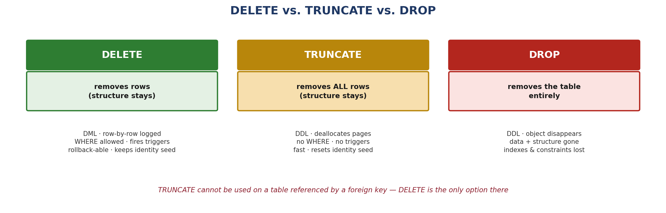
Figure 5.1 — Three different kinds of removal.

	DELETE	TRUNCATE	DROP
Category	DML	DDL	DDL
Removes	Selected rows	All rows	The whole object
WHERE clause	Yes	No	N/A
Logging	Each row logged	Page deallocations only	Minimal
Speed on large tables	Slow	Very fast	Very fast
Fires triggers	Yes	No	No
Resets IDENTITY	No	Yes	N/A
Blocked by inbound FK	No	Yes	Yes
Rollback in a transaction	Yes	Yes	Yes

-- DELETE: removes rows, keeps structure, can be filtered
DELETE FROM HR.Employees WHERE IsActive = 0;

-- TRUNCATE: removes every row, resets IDENTITY, cannot be filtered
TRUNCATE TABLE HR.EmployeeProjects;

-- DROP: removes the object entirely
DROP TABLE HR.EmployeeProjects;

-- Guarded drops (SQL Server 2016 and later)
DROP TABLE IF EXISTS HR.StagingEmployees;
DROP VIEW  IF EXISTS HR.vw_ActiveEmployees;

-- Older, portable guard
IF OBJECT_ID('HR.StagingEmployees', 'U') IS NOT NULL
    DROP TABLE HR.StagingEmployees;
GO

Both TRUNCATE and DROP are blocked while another table's foreign key references the target.

A frequent misconception is that TRUNCATE cannot be rolled back. Inside an explicit transaction it can — it is minimally logged, not unlogged. What cannot be recovered is a TRUNCATE that has already committed.

Best Practice: Choose appropriate data types and meaningful object names, and verify destructive DDL before execution.

Hands-On: Inside SQL_Training_DB, create the HR schema and the Departments, Employees, Projects, and EmployeeProjects tables using the exact columns and data types supplied. Then practise ALTER TABLE by adding a column, widening a column, and adding a CHECK constraint. Finally practise TRUNCATE and DROP on designated training objects only — never on the four core tables.

Module 6: SQL Syntax Basics

6.1 Anatomy of a Statement

SELECT     e.FirstName,                                -- column reference
           e.Salary * 1.10        AS NewSalary,        -- expression + alias
           'Reviewed'             AS ReviewStatus      -- literal + alias
FROM       HR.Employees AS e                           -- table + table alias
WHERE      e.DepartmentID = 3                          -- predicate
    AND    e.Salary > 40000
ORDER BY   e.Salary DESC;                              -- statement terminator

Keywords, identifiers, literals, expressions, aliases, comments — all six element types in one statement.

6.2 Keywords

Keywords are reserved words with defined meaning — SELECT, FROM, WHERE, JOIN. They are case-insensitive in SQL Server, but writing them in upper case is near-universal convention because it separates language from data at a glance.

A reserved word cannot be used as an identifier unless it is delimited. Avoiding reserved words as object names entirely is the better answer.

6.3 Identifiers

Identifiers name objects. Regular identifiers start with a letter, underscore, @ or #, contain only letters, digits, underscores, $, # or @, and are not reserved words. Anything else must be delimited with square brackets in T-SQL or double quotes in standard SQL.

-- Regular identifiers: no delimiters needed
SELECT EmployeeID, FirstName FROM HR.Employees;

-- Delimited identifiers: required for spaces or reserved words
SELECT [Employee ID], [Order] FROM dbo.[Order Details];

-- Fully qualified name: database.schema.object
SELECT * FROM SQL_Training_DB.HR.Employees;

-- Qualifying with the schema is the practical minimum
SELECT * FROM HR.Employees;       -- good: unambiguous, better plan reuse
SELECT * FROM Employees;          -- avoid: resolution depends on default schema

Always qualify with the schema. Unqualified names force an extra resolution step and can bind to the wrong object.

6.4 Literals

SELECT 42                        AS integer_literal,
       3.14                      AS decimal_literal,
       'Chennai'                 AS string_literal,
       N'नमस्ते'                   AS unicode_literal,     -- N prefix = NVARCHAR
       '2026-08-11'              AS date_literal,        -- ISO 8601, unambiguous
       'O''Brien'                AS escaped_quote,       -- doubled to escape
       1                         AS bit_true,
       NULL                      AS null_marker;

Always write dates as 'YYYY-MM-DD' — other formats are interpreted differently depending on server language settings.

6.5 Expressions and Operators

Operator group	Operators	Note
Arithmetic	`+ - * / %`	Integer / integer performs integer division
Comparison	`= <> != > < >= <=`	`<>` is the standard form of not-equal
Logical	AND OR NOT	AND binds tighter than OR — parenthesize
Range / set	BETWEEN, IN, LIKE, EXISTS	BETWEEN is inclusive of both endpoints
Null test	IS NULL, IS NOT NULL	Never use `= NULL`
String	`+` (T-SQL), CONCAT()	CONCAT ignores NULLs; `+` propagates them

-- Integer division is a classic trap
SELECT 7 / 2           AS integer_division,     -- 3, not 3.5
       7.0 / 2         AS decimal_division,     -- 3.500000
       7 * 1.0 / 2     AS forced_decimal;       -- 3.500000

-- Operator precedence: AND is evaluated before OR
SELECT * FROM HR.Employees
WHERE  DepartmentID = 1 OR DepartmentID = 2 AND Salary > 50000;
-- reads as: DepartmentID = 1 OR (DepartmentID = 2 AND Salary > 50000)

-- Parentheses make the intent explicit and correct
SELECT * FROM HR.Employees
WHERE  (DepartmentID = 1 OR DepartmentID = 2) AND Salary > 50000;

-- NULL propagation
SELECT 'A' + NULL                    AS concat_result,     -- NULL
       CONCAT('A', NULL)             AS concat_function,   -- 'A'
       ISNULL(NULL, 'fallback')      AS isnull_result;     -- 'fallback'

The two WHERE clauses above return different rows. This is one of the most common silent bugs in SQL.

6.6 Aliases

Aliases rename columns and tables for the duration of a query. Column aliases control the result heading; table aliases shorten references and are mandatory when a table is joined to itself.

-- Column aliases: AS is optional but recommended for clarity
SELECT FirstName + ' ' + LastName      AS FullName,
       Salary * 12                     AS AnnualSalary,
       Salary                          MonthlySalary       -- works, but less readable
FROM   HR.Employees AS e;

-- Aliases with spaces need delimiters
SELECT Salary * 12 AS [Annual Salary]
FROM   HR.Employees;

-- Table alias is required for a self-join
SELECT emp.FirstName   AS Employee,
       mgr.FirstName   AS Manager
FROM   HR.Employees AS emp
LEFT JOIN HR.Employees AS mgr ON emp.ManagerID = mgr.EmployeeID;

A column alias defined in SELECT cannot be reused in WHERE — WHERE is evaluated before SELECT.

6.7 Comments

-- Single-line comment: everything after the two dashes is ignored

/* Multi-line comment
   Useful for headers, disabling blocks,
   and documenting why a query exists. */

/*
    Purpose : Active headcount by department
    Author  : Training Team
    Created : 2026-08-11
    Notes   : Excludes contractors (IsActive flag only covers permanent staff)
*/
SELECT DepartmentID,
       COUNT(*) AS HeadCount
FROM   HR.Employees
WHERE  IsActive = 1            -- excludes leavers
GROUP  BY DepartmentID;

Comment why, not what. The SQL already says what it does.

6.8 Batches and GO

GO is not a SQL statement — it is a batch separator understood by SSMS and sqlcmd, not by the database engine. It tells the client to send everything above it as one batch. Some statements, such as CREATE SCHEMA, CREATE VIEW, and CREATE PROCEDURE, must be the first statement in their batch, which is why GO appears between them.

Variables declared in one batch do not survive into the next.

6.9 Formatting Conventions

-- Hard to read: no structure, no qualification, unclear intent
select e.firstname,d.departmentname,e.salary from hr.employees e join
hr.departments d on e.departmentid=d.departmentid where e.salary>50000 and
e.isactive=1 order by e.salary desc;

-- Readable: keywords upper case, one clause per line, aligned, aliased
SELECT      e.FirstName,
            d.DepartmentName,
            e.Salary
FROM        HR.Employees      AS e
INNER JOIN  HR.Departments    AS d
        ON  e.DepartmentID = d.DepartmentID
WHERE       e.Salary   > 50000
    AND     e.IsActive = 1
ORDER BY    e.Salary DESC;

Both queries produce identical results and identical execution plans. Only one can be reviewed quickly.

Keywords upper case, identifiers in their declared case: the eye separates language from data instantly.
One clause per line: SELECT, FROM, WHERE, GROUP BY, ORDER BY each start a new line.
One column per line in long SELECT lists: makes diffs in version control readable.
Indent continuations and join conditions: shows what belongs to what.
Always qualify columns in multi-table queries: e.Salary, not Salary — removes ambiguity and survives schema changes.
Terminate statements with a semicolon: optional in T-SQL today, required for some constructs, and mandatory in standard SQL.

Best Practice: Write SQL consistently, indent queries, and avoid ambiguous object names.

Module 7: SQL Naming Conventions

7.1 General Rules

Be descriptive: HireDate, not HD or Date1.
Avoid unclear abbreviations: Amount over Amt, CustomerID over CustID. Abbreviate only what the whole organization already abbreviates.
No spaces or special characters: they force delimiters on every reference forever.
Never use reserved words: Order, User, Date, Key, Table, Group are all traps.
No type prefixes on tables: tbl_Employees adds nothing; the object type is already known.
Pick one case style: PascalCase (EmployeeID) or snake_case (employee_id). Never mix.
Be consistent about plurality: either all tables plural (Employees) or all singular (Employee).

7.2 Object Naming Standards

Object	Convention	Example
Database	PascalCase, purpose-describing	SQL_Training_DB, SalesReporting
Schema	Short business area	HR, Sales, Finance, Staging
Table	PascalCase noun, consistent plurality	Employees, Departments
Column	PascalCase, no table prefix	FirstName, HireDate, Salary
Primary key	PK_TableName	PK_Employees
Foreign key	FK_ChildTable_ParentTable	FK_Employees_Departments
Unique	UQ_TableName_Column	UQ_Employees_Email
Check	CK_TableName_Rule	CK_Employees_Salary
Default	DF_TableName_Column	DF_Employees_IsActive
Index	IX_TableName_Columns	IX_Employees_DepartmentID
View	vw_Purpose	vw_ActiveEmployees
Stored procedure	usp_VerbNoun	usp_GetEmployeesByDept
Function	fn_Purpose	fn_CalculateAnnualSalary
Trigger	TR_TableName_Action	TR_Employees_AfterInsert

Prefixes on constraints and indexes are worth the characters: when a violation is raised at two in the morning, FK_Employees_Departments identifies the problem instantly while FK__Employe__3B75D760 does not.

7.3 Named vs. Auto-Generated Constraints

-- Auto-generated name: SQL Server invents something unreadable
CREATE TABLE HR.BadExample
(
    ID    INT PRIMARY KEY,                   -- becomes PK__BadExamp__3213E83F1A2B3C4D
    Email NVARCHAR(150) UNIQUE               -- becomes UQ__BadExamp__A9D10534...
);

-- Explicitly named: readable, and identical across every environment
CREATE TABLE HR.GoodExample
(
    ID    INT           NOT NULL,
    Email NVARCHAR(150) NULL,

    CONSTRAINT PK_GoodExample PRIMARY KEY (ID),
    CONSTRAINT UQ_GoodExample_Email UNIQUE (Email)
);
GO

Auto-generated names differ between environments, so scripts that reference them break on deployment.

7.4 Naming Applied

-- Poor naming: opaque, inconsistent, reserved words, forced delimiters
CREATE TABLE dbo.tbl_emp1
(
    id      INT,
    [name]  VARCHAR(50),
    dt      DATETIME,
    [desc]  VARCHAR(200),
    flag    BIT,
    amt     FLOAT
);

-- Good naming: self-documenting and consistent
CREATE TABLE HR.Employees
(
    EmployeeID      INT            NOT NULL IDENTITY(1,1),
    FullName        NVARCHAR(100)  NOT NULL,
    HireDate        DATE           NOT NULL,
    JobDescription  NVARCHAR(200)  NULL,
    IsActive        BIT            NOT NULL,
    AnnualSalary    DECIMAL(12,2)  NOT NULL,

    CONSTRAINT PK_Employees PRIMARY KEY (EmployeeID)
);
GO

The second table needs no documentation — the names and types are the documentation.

Best Practice: Follow one organization-wide naming convention consistently, use meaningful names, and avoid unclear abbreviations.

Module 8: SQL Command Categories

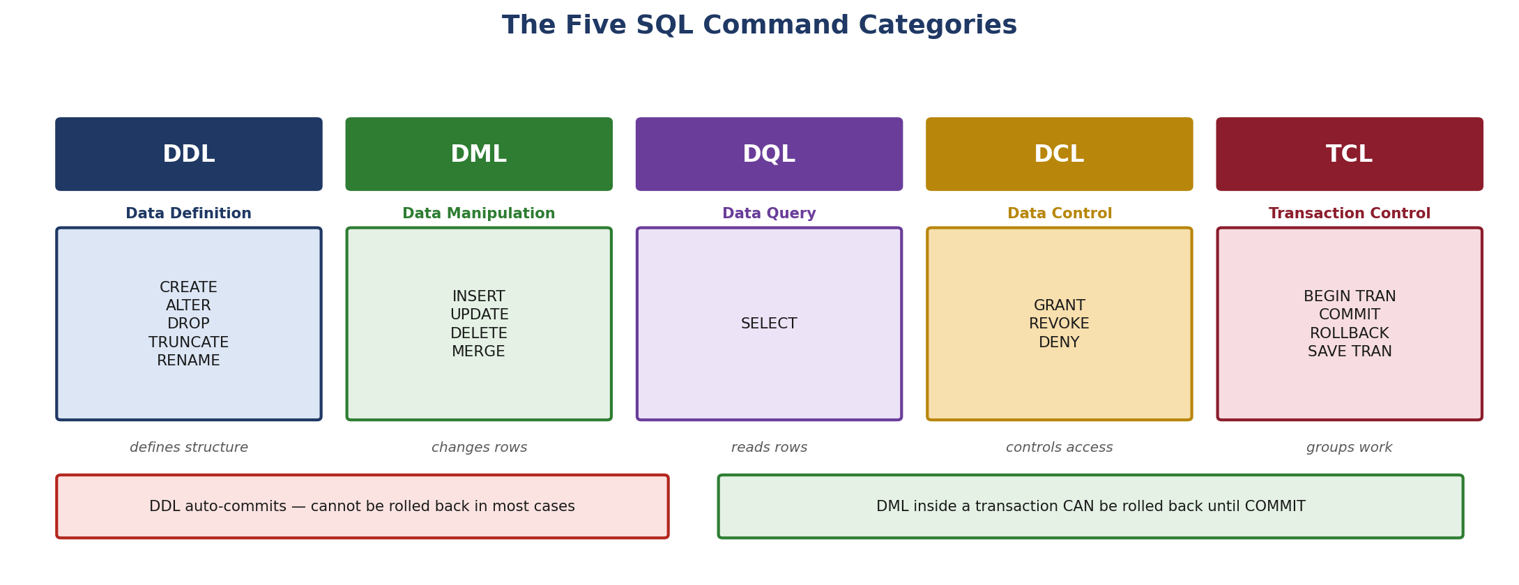
Figure 8.1 — The five categories and their commands.

8.1 DDL — Data Definition Language

DDL defines and modifies structure. In SQL Server, DDL statements auto-commit: each one becomes permanent the moment it succeeds, unless explicitly wrapped in a transaction.

CREATE TABLE   HR.Locations (LocationID INT PRIMARY KEY, City NVARCHAR(50));
ALTER  TABLE   HR.Locations ADD Country NVARCHAR(50) NULL;
TRUNCATE TABLE HR.Locations;
DROP   TABLE   HR.Locations;

CREATE, ALTER, DROP, TRUNCATE — structure in, structure out.

8.2 DML — Data Manipulation Language

DML changes the rows inside existing structures. Every DML statement is fully logged and can be rolled back while its transaction remains open.

INSERT INTO HR.Departments (DepartmentName, Location)
VALUES ('Analytics', 'Chennai');

UPDATE HR.Employees
SET    Salary = Salary * 1.10
WHERE  DepartmentID = 3;

DELETE FROM HR.Employees
WHERE  IsActive = 0;

INSERT, UPDATE, DELETE (and MERGE) — rows in, rows out.

8.3 DQL — Data Query Language

DQL retrieves data without changing it. It contains a single statement, SELECT, which is nonetheless the largest and most-used part of SQL. Many texts fold DQL into DML; separating it is clearer because reading and writing carry entirely different risks.

SELECT      d.DepartmentName,
            COUNT(*)          AS HeadCount,
            AVG(e.Salary)     AS AverageSalary
FROM        HR.Employees   AS e
INNER JOIN  HR.Departments AS d ON e.DepartmentID = d.DepartmentID
WHERE       e.IsActive = 1
GROUP BY    d.DepartmentName
HAVING      COUNT(*) > 2
ORDER BY    AverageSalary DESC;

SELECT reads data and never modifies it.

8.4 DCL — Data Control Language

DCL manages permissions. GRANT gives a right, REVOKE removes a previously granted right, and DENY blocks a right outright — DENY overrides any GRANT, including one inherited through a role.

GRANT  SELECT, INSERT ON HR.Employees TO training_user;
REVOKE INSERT ON HR.Employees FROM training_user;
DENY   DELETE ON HR.Employees TO training_user;

-- Schema-wide grant
GRANT SELECT ON SCHEMA::HR TO training_user;

-- Review effective permissions
SELECT pr.name                   AS principal_name,
       pe.permission_name,
       pe.state_desc,            -- GRANT, REVOKE, DENY
       OBJECT_NAME(pe.major_id)  AS object_name
FROM   sys.database_permissions  AS pe
JOIN   sys.database_principals   AS pr ON pe.grantee_principal_id = pr.principal_id
WHERE  pr.name = 'training_user';

REVOKE removes a permission entry; DENY actively blocks. They are not the same.

8.5 TCL — Transaction Control Language

TCL groups statements into transactions so they succeed or fail as a unit. This is what makes multi-step operations safe.

BEGIN TRANSACTION;

    UPDATE HR.Employees
    SET    DepartmentID = 4
    WHERE  EmployeeID = 1001;

    -- Verify before deciding
    SELECT EmployeeID, DepartmentID FROM HR.Employees WHERE EmployeeID = 1001;

    -- If correct:
    COMMIT TRANSACTION;
    -- If not:
    -- ROLLBACK TRANSACTION;
GO

-- Savepoints allow partial rollback within one transaction
BEGIN TRANSACTION;
    INSERT INTO HR.Departments (DepartmentName) VALUES ('Temp A');
    SAVE TRANSACTION AfterFirstInsert;

    INSERT INTO HR.Departments (DepartmentName) VALUES ('Temp B');
    ROLLBACK TRANSACTION AfterFirstInsert;   -- undoes only 'Temp B'
COMMIT TRANSACTION;                          -- 'Temp A' is kept
GO

A transaction left open holds locks until committed or rolled back — never leave BEGIN TRANSACTION unfinished.

8.6 Comparing the Categories

	DDL	DML	DQL	DCL	TCL
Affects	Structure	Rows	Nothing	Permissions	Transactions
Auto-commits	Yes	No	N/A	Yes	N/A
Rollback-able	Limited	Yes	N/A	Limited	Is the mechanism
Fully logged	Metadata	Yes	No	Metadata	Yes
Typical user	Developer / DBA	Developer / app	Analyst	DBA	Developer

8.7 Classification Reference

Command	Category	Command	Category
CREATE TABLE	DDL	GRANT	DCL
ALTER TABLE	DDL	REVOKE	DCL
DROP TABLE	DDL	DENY	DCL
TRUNCATE TABLE	DDL	BEGIN TRANSACTION	TCL
CREATE INDEX	DDL	COMMIT	TCL
CREATE VIEW	DDL	ROLLBACK	TCL
ALTER DATABASE	DDL	SAVE TRANSACTION	TCL
INSERT	DML	SELECT	DQL
UPDATE	DML	SELECT ... INTO	DQL / DDL hybrid
DELETE	DML	CREATE PROCEDURE	DDL
MERGE	DML	DROP VIEW	DDL
BULK INSERT	DML	ALTER SCHEMA	DDL

Best Practice: Understand the impact of a command category before execution, particularly DDL, DML, and TCL.

Hands-On: Classify the following 25 commands into DDL, DML, DQL, DCL, or TCL: CREATE TABLE, INSERT, SELECT, GRANT, COMMIT, ALTER TABLE, UPDATE, REVOKE, ROLLBACK, DROP TABLE, DELETE, DENY, SAVE TRANSACTION, TRUNCATE TABLE, MERGE, BEGIN TRANSACTION, CREATE INDEX, BULK INSERT, CREATE VIEW, ALTER DATABASE, DROP INDEX, CREATE PROCEDURE, SELECT INTO, ALTER SCHEMA, and SET TRANSACTION ISOLATION LEVEL. For each, also state whether it auto-commits.

Module 9: Basic Data Operations – DML

9.1 INSERT

-- Named columns: the only form that should appear in real code
INSERT INTO HR.Departments (DepartmentName, Location)
VALUES ('Analytics', 'Chennai');

-- Multiple rows in one statement
INSERT INTO HR.Departments (DepartmentName, Location)
VALUES ('Engineering', 'Bengaluru'),
       ('Finance',     'Mumbai'),
       ('Operations',  'Chennai');

-- Positional insert: works, but breaks the moment a column is added
INSERT INTO HR.Departments VALUES ('Legal', 'Delhi', SYSDATETIME());   -- avoid

Always list the target columns. Positional INSERT is a latent bug waiting for the next ALTER TABLE.

-- Insert into a table with IDENTITY: never supply the identity value
INSERT INTO HR.Employees
    (FirstName, LastName, Email, HireDate, Salary, DepartmentID, IsActive)
VALUES
    ('Ravi',  'Kumar', 'ravi.kumar@example.com',  '2026-01-15', 55000.00, 1, 1),
    ('Meera', 'Nair',  'meera.nair@example.com',  '2026-02-01', 62000.00, 2, 1),
    ('Arjun', 'Rao',   'arjun.rao@example.com',   '2026-03-10', 48000.00, 1, 1);

-- Retrieve the identity value just generated
SELECT SCOPE_IDENTITY() AS LastInsertedEmployeeID;

-- Copy rows from a query result
INSERT INTO HR.EmployeeArchive (EmployeeID, FullName, ArchivedOn)
SELECT EmployeeID,
       FirstName + ' ' + LastName,
       SYSDATETIME()
FROM   HR.Employees
WHERE  IsActive = 0;

-- Capture what was inserted
INSERT INTO HR.Departments (DepartmentName, Location)
OUTPUT inserted.DepartmentID, inserted.DepartmentName
VALUES ('Quality Assurance', 'Pune');

SCOPE_IDENTITY() is the safe choice; @@IDENTITY can return a value generated by a trigger.

9.2 UPDATE

UPDATE without a WHERE clause modifies every row in the table. There is no confirmation prompt. This single omission causes more production incidents than any other SQL mistake.

-- STEP 1 - always: run the WHERE clause as a SELECT first
SELECT EmployeeID, FirstName, Salary
FROM   HR.Employees
WHERE  DepartmentID = 3;              -- confirm the row count and the rows

-- STEP 2: run the UPDATE with the identical WHERE clause
UPDATE HR.Employees
SET    Salary = Salary * 1.10
WHERE  DepartmentID = 3;

-- STEP 3: verify the result
SELECT EmployeeID, FirstName, Salary
FROM   HR.Employees
WHERE  DepartmentID = 3;

The SELECT-first pattern costs three seconds and prevents the most expensive class of error.

-- Update several columns at once
UPDATE HR.Employees
SET    Email        = 'ravi.k@example.com',
       DepartmentID = 2,
       IsActive     = 1
WHERE  EmployeeID   = 1001;

-- Update using a value from another table
UPDATE e
SET    e.Salary = e.Salary * 1.05
FROM   HR.Employees   AS e
INNER JOIN HR.Departments AS d ON e.DepartmentID = d.DepartmentID
WHERE  d.DepartmentName = 'Analytics';

-- Capture before-and-after values
UPDATE HR.Employees
SET    Salary = Salary * 1.10
OUTPUT deleted.EmployeeID,
       deleted.Salary  AS OldSalary,
       inserted.Salary AS NewSalary
WHERE  DepartmentID = 3;

-- Safest form for anything irreversible
BEGIN TRANSACTION;
    UPDATE HR.Employees SET Salary = Salary * 1.10 WHERE DepartmentID = 3;
    PRINT CONCAT(@@ROWCOUNT, ' rows affected');   -- expected number?
    -- COMMIT TRANSACTION;
    -- ROLLBACK TRANSACTION;
GO

@@ROWCOUNT after the statement is the fastest sanity check available.

9.3 DELETE

-- STEP 1: confirm exactly which rows will go
SELECT EmployeeID, FirstName, LastName, IsActive
FROM   HR.Employees
WHERE  IsActive = 0;

-- STEP 2: delete with the identical predicate
DELETE FROM HR.Employees
WHERE  IsActive = 0;

-- STEP 3: verify
SELECT COUNT(*) AS RemainingInactive
FROM   HR.Employees
WHERE  IsActive = 0;

-- Delete specific test records by ID
DELETE FROM HR.Employees
WHERE  EmployeeID IN (9001, 9002, 9003);

-- Keep a record of what was removed
DELETE FROM HR.Employees
OUTPUT deleted.EmployeeID, deleted.FirstName, deleted.LastName
WHERE  EmployeeID = 9004;

-- DELETE without WHERE removes every row - almost never intended
-- DELETE FROM HR.Employees;

A DELETE blocked by a foreign key is the database protecting referential integrity, not an error to work around.

9.4 Safety Rules for DML

Confirm the database context: run SELECT DB_NAME() before anything else.
Write the WHERE clause first: some practitioners literally type the WHERE before the UPDATE to avoid an accidental execution.
Test with SELECT: run the exact predicate as a SELECT and check the row count.
Wrap in a transaction: BEGIN TRANSACTION, verify, then COMMIT or ROLLBACK.
Check @@ROWCOUNT: if you expected 5 rows and 5,000 changed, roll back.
Never highlight-and-run part of a script: executing a selection can run an UPDATE without its WHERE clause.
Prefer soft deletes where history matters: set IsActive = 0 rather than removing the row.

Best Practice: Always verify WHERE conditions before UPDATE or DELETE, and test with SELECT first.

Hands-On: Insert the supplied sample employee records into HR.Employees. Update the records matching the explicitly provided IDs and conditions. Delete the specified test records. Before and after each modification, run a SELECT to verify the affected rows, and record the @@ROWCOUNT for each statement.

Module 10: Basic SELECT – DQL

10.1 Structure of a SELECT

SELECT     column_list          -- 5. which columns to return
FROM       table_source         -- 1. where the rows come from
WHERE      row_filter           -- 2. which rows qualify
GROUP BY   grouping_columns     -- 3. how rows are collapsed
HAVING     group_filter         -- 4. which groups qualify
ORDER BY   sort_columns;        -- 6. how the result is sorted

Written order and logical processing order differ — the numbers show the order the engine actually applies.

This ordering explains a rule that otherwise looks arbitrary: a column alias defined in SELECT cannot be used in WHERE, because WHERE runs before SELECT exists. It can be used in ORDER BY, which runs after.

-- Fails: AnnualSalary does not exist yet when WHERE is evaluated
-- SELECT Salary * 12 AS AnnualSalary
-- FROM   HR.Employees
-- WHERE  AnnualSalary > 600000;

-- Works: repeat the expression in WHERE
SELECT Salary * 12 AS AnnualSalary
FROM   HR.Employees
WHERE  Salary * 12 > 600000;

-- Works: ORDER BY runs after SELECT, so the alias is available
SELECT Salary * 12 AS AnnualSalary
FROM   HR.Employees
ORDER  BY AnnualSalary DESC;

The same rule explains why aggregate filters go in HAVING rather than WHERE.

10.2 Selecting Columns

-- Every column: convenient in exploration, wrong in production code
SELECT * FROM HR.Employees;

-- Named columns: return only what is needed
SELECT EmployeeID,
       FirstName,
       LastName,
       Salary
FROM   HR.Employees;

-- Qualified columns in a multi-table query
SELECT      e.EmployeeID,
            e.FirstName,
            d.DepartmentName
FROM        HR.Employees   AS e
INNER JOIN  HR.Departments AS d ON e.DepartmentID = d.DepartmentID;

SELECT * is fine at the SSMS prompt and a liability in a saved report or view.

Why SELECT * Is Avoided in Production

Unnecessary I/O and network traffic: columns you never read are still fetched and transmitted.
It defeats covering indexes: an index that could have satisfied the query is bypassed once every column is demanded.
It breaks silently on schema change: adding or reordering a column changes the result shape and can break downstream code.
It hides intent: a reader cannot tell which columns the logic actually depends on.

10.3 Column Aliases

SELECT EmployeeID                      AS ID,
       FirstName                       AS [First Name],
       LastName                        AS [Last Name],
       Salary                          AS MonthlySalary,
       Salary * 12                     AS AnnualSalary
FROM   HR.Employees;

-- Table aliases shorten every reference
SELECT      e.FirstName,
            d.DepartmentName
FROM        HR.Employees   AS e
INNER JOIN  HR.Departments AS d ON e.DepartmentID = d.DepartmentID;

Use AS explicitly and delimit any alias containing spaces.

10.4 Expressions and Computed Columns

SELECT EmployeeID,

       -- String concatenation
       FirstName + ' ' + LastName                        AS FullName,
       CONCAT(FirstName, ' ', LastName)                  AS FullNameSafe,

       -- Arithmetic
       Salary                                            AS MonthlySalary,
       Salary * 12                                       AS AnnualSalary,
       ROUND(Salary * 0.10, 2)                           AS MonthlyTax,

       -- Date arithmetic
       HireDate,
       DATEDIFF(YEAR, HireDate, GETDATE())               AS YearsOfService,
       DATEADD(YEAR, 1, HireDate)                        AS FirstAnniversary,

       -- Conditional logic
       CASE
           WHEN Salary >= 70000 THEN 'Senior'
           WHEN Salary >= 50000 THEN 'Mid'
           ELSE 'Junior'
       END                                               AS SalaryBand,

       -- NULL handling
       ISNULL(Email, 'no-email-on-file')                 AS EmailOrDefault,
       COALESCE(ManagerID, EmployeeID)                   AS EffectiveManagerID

FROM   HR.Employees;

CONCAT treats NULL as an empty string; the + operator returns NULL if any operand is NULL.

10.5 DISTINCT

DISTINCT removes duplicate rows from the result. It applies to the entire selected row, not to one column — a frequent misunderstanding.

-- Distinct values of a single column
SELECT DISTINCT DepartmentID
FROM   HR.Employees;

-- DISTINCT applies to the whole row: this returns unique COMBINATIONS
SELECT DISTINCT DepartmentID, IsActive
FROM   HR.Employees;

-- Counting distinct values
SELECT COUNT(*)                        AS TotalEmployees,
       COUNT(DISTINCT DepartmentID)    AS DepartmentsRepresented,
       COUNT(Email)                    AS EmployeesWithEmail    -- NULLs excluded
FROM   HR.Employees;

COUNT(*) counts rows; COUNT(column) counts non-NULL values in that column.

DISTINCT requires a sort or hash to identify duplicates, so it is not free. If duplicates are appearing unexpectedly in a joined query, the usual cause is the join itself — fix the join rather than masking it with DISTINCT.

10.6 Filtering, Sorting, and Limiting

-- WHERE: filter rows
SELECT FirstName, Salary
FROM   HR.Employees
WHERE  Salary BETWEEN 40000 AND 70000          -- inclusive of both bounds
   AND DepartmentID IN (1, 2, 3)
   AND LastName LIKE 'K%'                      -- starts with K
   AND Email IS NOT NULL;

-- ORDER BY: sort the result
SELECT FirstName, Salary
FROM   HR.Employees
ORDER  BY Salary DESC, LastName ASC;

-- TOP: limit the number of rows (T-SQL)
SELECT TOP 5 FirstName, Salary
FROM   HR.Employees
ORDER  BY Salary DESC;                          -- TOP without ORDER BY is meaningless

SELECT TOP 10 PERCENT FirstName, Salary
FROM   HR.Employees
ORDER  BY Salary DESC;

-- Standard-SQL paging, portable and preferred for pagination
SELECT      FirstName, Salary
FROM        HR.Employees
ORDER BY    Salary DESC
OFFSET      10 ROWS
FETCH NEXT  10 ROWS ONLY;

Without ORDER BY, row order is not guaranteed — even if it looks stable in testing.

10.7 A Complete Query

/*
    Purpose : Active employees with salary band and tenure, highest paid first
    Author  : Training Team
    Created : 2026-08-11
*/
SELECT      e.EmployeeID,
            e.FirstName + ' ' + e.LastName              AS FullName,
            d.DepartmentName,
            e.Salary                                    AS MonthlySalary,
            e.Salary * 12                               AS AnnualSalary,
            DATEDIFF(YEAR, e.HireDate, GETDATE())       AS YearsOfService,
            CASE
                WHEN e.Salary >= 70000 THEN 'Senior'
                WHEN e.Salary >= 50000 THEN 'Mid'
                ELSE 'Junior'
            END                                         AS SalaryBand,
            ISNULL(e.Email, 'not provided')             AS ContactEmail
FROM        HR.Employees   AS e
INNER JOIN  HR.Departments AS d
        ON  e.DepartmentID = d.DepartmentID
WHERE       e.IsActive = 1
    AND     e.Salary   > 40000
ORDER BY    e.Salary DESC;

Named columns, qualified references, explicit aliases, documented purpose — production-shaped SQL.

Best Practice: Avoid SELECT * in production queries and retrieve only the columns you need.

Hands-On: Write queries to retrieve the specified columns from HR.Employees, rename them using aliases, build the supplied expressions (full name, annual salary, years of service, salary band), apply DISTINCT where required, and compare each result against the provided expected output. For every query, state why you selected the columns you did instead of using SELECT *.

Phase 4 – Filtering and Working with Data

Phase 4 Overview

Every script in this phase is directly runnable. Scripts assume SQL Server and the HR schema created in Phase 3.

#	Subtopic	Learning Outcome
1	SQL Query Order of Execution	Logical processing sequence and how each clause feeds the next
2	Filtering Data	WHERE, comparisons, AND/OR/NOT, BETWEEN, IN, LIKE, NULL checks
3	Sorting & Limiting Results	ORDER BY, ASC/DESC, TOP, OFFSET, FETCH, LIMIT
4	SQL Operators	Arithmetic, comparison, logical, and concatenation operators
5	Working with NULL	NULL semantics, IS NULL, IS NOT NULL, COALESCE and related functions

Module 1: SQL Query Order of Execution

1.1 Written Order vs. Logical Order

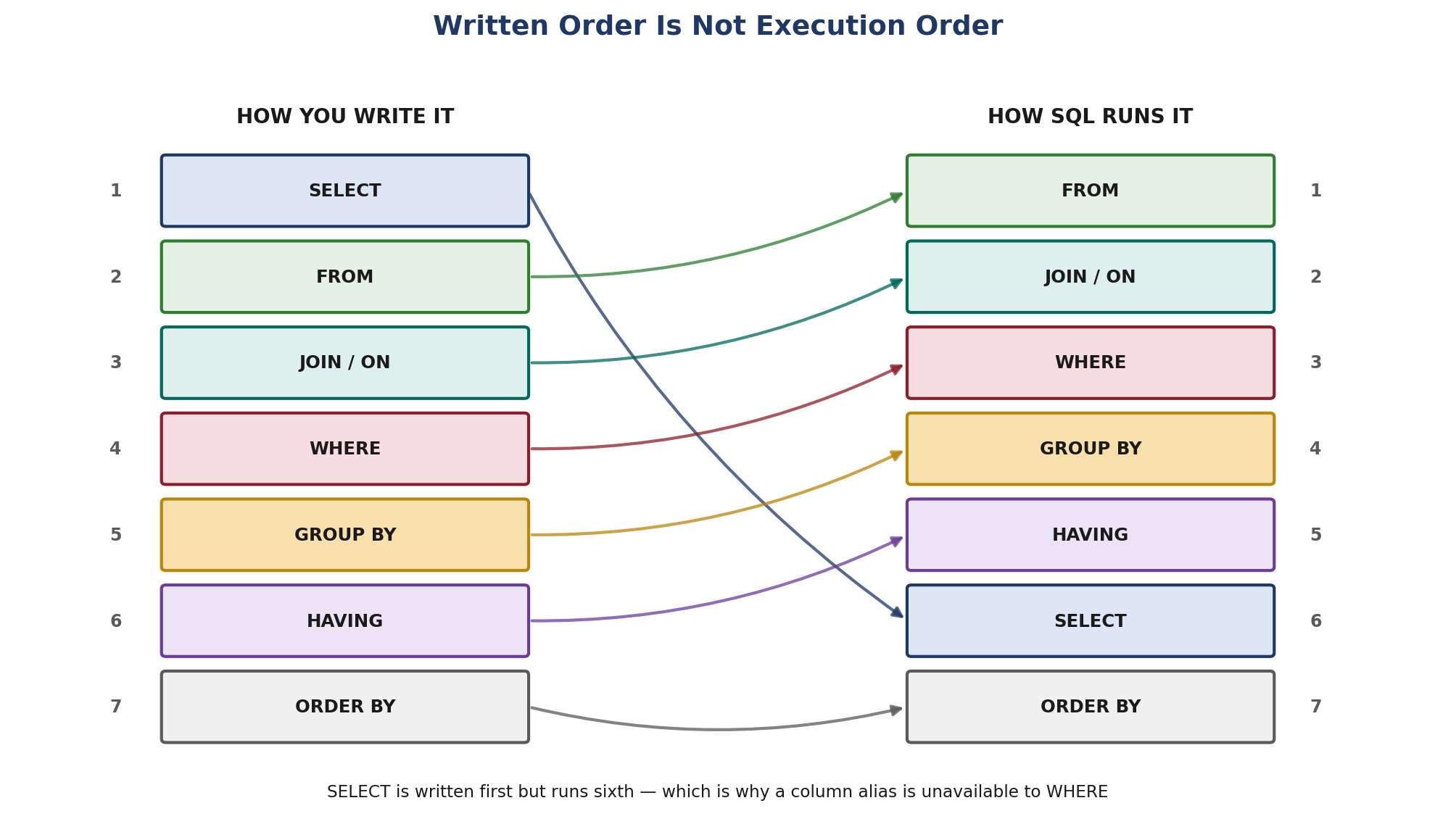
Figure 1.1 — The same seven clauses, in two different orders.

Written position	Clause	Logical position	What it does
1	SELECT	6	Chooses columns, evaluates expressions, creates aliases
2	FROM	1	Identifies the source table
3	JOIN / ON	2	Combines tables and filters the combination
4	WHERE	3	Filters individual rows
5	GROUP BY	4	Collapses rows into groups
6	HAVING	5	Filters the groups
7	ORDER BY	7	Sorts the final result

1.2 The Full Logical Sequence

Written out completely, the engine processes a query in this order. Each step produces an intermediate result that the next step consumes.

FROM: the source table is identified and its rows are read.
ON: the join predicate is evaluated to decide which row combinations match.
JOIN: unmatched rows are added back for OUTER joins.
WHERE: individual rows are filtered. Aggregates cannot be referenced here.
GROUP BY: surviving rows collapse into one row per distinct grouping value.
HAVING: whole groups are filtered. Aggregates can be referenced here.
SELECT: columns are chosen, expressions evaluated, aliases created.
DISTINCT: duplicate rows are removed from the projected result.
ORDER BY: the result is sorted. Aliases from SELECT are available here.
TOP / OFFSET-FETCH: the row count is limited, last of all.

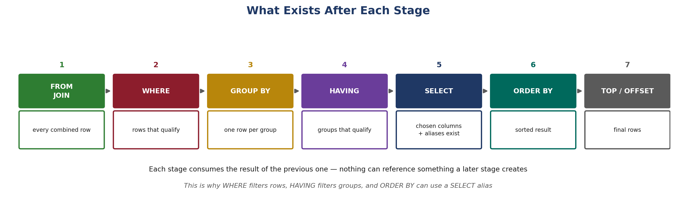
Figure 1.2 — What exists after each stage.

1.3 Consequence One: Aliases in WHERE

A column alias is created at step 7, but WHERE runs at step 4. At the moment WHERE is evaluated, the alias does not exist yet, so referencing it raises an invalid column name error.

SELECT FirstName,
       Salary * 12 AS AnnualSalary
FROM   HR.Employees
WHERE  AnnualSalary > 600000;

This query fails. AnnualSalary is created by SELECT, which has not run when WHERE is evaluated.

There are two correct fixes. Repeat the expression in WHERE, or wrap the query so the alias exists in an outer scope.

SELECT FirstName,
       Salary * 12 AS AnnualSalary
FROM   HR.Employees
WHERE  Salary * 12 > 600000;

Repeating the expression is the simplest fix and costs nothing at runtime.

SELECT FirstName,
       AnnualSalary
FROM
(
    SELECT FirstName,
           Salary * 12 AS AnnualSalary
    FROM   HR.Employees
) AS e
WHERE  e.AnnualSalary > 600000;

A derived table makes the alias available because the inner query completes first.

1.4 Consequence Two: Aliases in ORDER BY Work

ORDER BY runs at step 9, after SELECT. By then the alias exists, so it can be used freely.

SELECT      FirstName,
            Salary * 12 AS AnnualSalary
FROM        HR.Employees
ORDER BY    AnnualSalary DESC;

Valid. ORDER BY is the only clause that can see a SELECT alias.

1.5 Consequence Three: WHERE vs. HAVING

WHERE filters rows before grouping. HAVING filters groups after grouping. Because WHERE runs at step 4 and GROUP BY at step 5, an aggregate cannot appear in WHERE — no groups exist yet.

SELECT      DepartmentID,
            COUNT(*) AS HeadCount
FROM        HR.Employees
WHERE       COUNT(*) > 5
GROUP BY    DepartmentID;

This query fails. COUNT(*) is not available at the WHERE stage.

SELECT      DepartmentID,
            COUNT(*) AS HeadCount
FROM        HR.Employees
GROUP BY    DepartmentID
HAVING      COUNT(*) > 5;

Correct. HAVING runs after GROUP BY, so aggregates are available.

Both clauses are often needed together, and each does a different job. Filtering with WHERE first is also faster, because fewer rows reach the grouping stage.

SELECT      DepartmentID,
            COUNT(*)        AS HeadCount,
            AVG(Salary)     AS AverageSalary
FROM        HR.Employees
WHERE       IsActive = 1
GROUP BY    DepartmentID
HAVING      COUNT(*) > 5
        AND AVG(Salary) > 50000
ORDER BY    AverageSalary DESC;

WHERE removes inactive employees; HAVING removes small or low-paying departments.

1.6 Consequence Four: SELECT Columns and GROUP BY

After GROUP BY, only two things exist: the grouping columns and aggregates over them. Any other column has no single value for the group, so referencing it is an error.

SELECT      DepartmentID,
            FirstName,
            COUNT(*) AS HeadCount
FROM        HR.Employees
GROUP BY    DepartmentID;

This query fails. FirstName has many values per department and is not in GROUP BY.

SELECT      DepartmentID,
            COUNT(*)        AS HeadCount,
            MIN(FirstName)  AS SampleName
FROM        HR.Employees
GROUP BY    DepartmentID;

Valid. An aggregate reduces the many values to one.

1.7 Consequence Five: DISTINCT and ORDER BY

DISTINCT runs at step 8, after SELECT and before ORDER BY. A query cannot sort by a column that DISTINCT has already discarded, because that column is no longer part of the result.

SELECT DISTINCT DepartmentID
FROM     HR.Employees
ORDER BY HireDate;

This query fails. HireDate is not in the DISTINCT result, so it cannot be sorted on.

SELECT DISTINCT DepartmentID
FROM     HR.Employees
ORDER BY DepartmentID;

Valid. Only columns that survive DISTINCT can be sorted.

1.8 Tracing a Query Stage by Stage

The best way to internalize the sequence is to walk one query through it and name the intermediate result at each point.

SELECT      d.DepartmentName,
            COUNT(*)          AS HeadCount,
            AVG(e.Salary)     AS AverageSalary
FROM        HR.Employees   AS e
INNER JOIN  HR.Departments AS d
        ON  e.DepartmentID = d.DepartmentID
WHERE       e.IsActive = 1
        AND e.Salary   > 30000
GROUP BY    d.DepartmentName
HAVING      COUNT(*) >= 3
ORDER BY    AverageSalary DESC;

The query below is processed in the sequence described in the table that follows.

Step	Clause	Intermediate result
1	FROM HR.Employees	All employee rows
2	ON e.DepartmentID = d.DepartmentID	Matching employee-department pairs
3	INNER JOIN	Only matched pairs kept
4	WHERE	Active employees earning over 30000
5	GROUP BY d.DepartmentName	One row per department
6	`HAVING COUNT(*) >= 3`	Only departments with 3 or more employees
7	SELECT	DepartmentName, HeadCount, AverageSalary
8	ORDER BY AverageSalary DESC	Sorted using the alias created in step 7

1.9 Debugging with the Sequence

Error or symptom	Stage responsible	Fix
Invalid column name on an alias	Alias used before SELECT ran	Repeat the expression, or use a derived table
Aggregate not allowed in WHERE	WHERE runs before GROUP BY	Move the condition to HAVING
Column invalid in the select list	Not grouped and not aggregated	Add to GROUP BY or wrap in an aggregate
ORDER BY item not in DISTINCT list	DISTINCT ran first	Sort only by surviving columns
Outer join behaving like an inner join	Condition placed in WHERE, not ON	Move the predicate into the ON clause
TOP returns unexpected rows	TOP applies last, after ORDER BY	Add a deterministic ORDER BY

Best Practice: Use the logical execution order when debugging, especially for issues involving aliases, filtering, grouping, and aggregation.

Hands-On: Work through 5–10 supplied queries containing SELECT, FROM, JOIN, WHERE, GROUP BY, HAVING, and ORDER BY. For each: write out the logical execution sequence, predict the intermediate result after each stage, and state the expected row count. Then repair the supplied broken queries — those using an alias in WHERE, an aggregate in WHERE, an ungrouped column in SELECT, and an outer-join predicate in the wrong clause — explaining which stage caused each failure.

Module 2: Filtering Data

2.1 Comparison Operators

Operator	Meaning	Example
`=`	Equal to	`WHERE DepartmentID = 3`
`<>` or `!=`	Not equal to	`WHERE DepartmentID <> 3`
`>`	Greater than	`WHERE Salary > 50000`
`<`	Less than	`WHERE Salary < 50000`
`>=`	Greater than or equal to	`WHERE Salary >= 50000`
`<=`	Less than or equal to	`WHERE HireDate <= '2026-01-01'`

SELECT EmployeeID, FirstName, Salary
FROM   HR.Employees
WHERE  Salary = 50000;

SELECT EmployeeID, FirstName, DepartmentID
FROM   HR.Employees
WHERE  DepartmentID <> 3;

SELECT EmployeeID, FirstName, Salary
FROM   HR.Employees
WHERE  Salary > 50000;

SELECT EmployeeID, FirstName, HireDate
FROM   HR.Employees
WHERE  HireDate >= '2026-01-01';

<> is the standard form of not-equal; != is accepted by SQL Server but is not portable.

2.2 Combining Conditions with AND, OR, NOT

AND requires every condition to be true. OR requires at least one. NOT inverts a condition. Crucially, AND is evaluated before OR, which is the source of a great many silent logic bugs.

SELECT EmployeeID, FirstName, Salary, DepartmentID
FROM   HR.Employees
WHERE  DepartmentID = 1
   AND Salary > 45000;

SELECT EmployeeID, FirstName, DepartmentID
FROM   HR.Employees
WHERE  DepartmentID = 1
    OR DepartmentID = 2;

SELECT EmployeeID, FirstName, IsActive
FROM   HR.Employees
WHERE  NOT IsActive = 1;

Three basic combinations: all conditions, any condition, and negation.

Why Parentheses Matter

The next two queries look almost identical and return different rows. In the first, AND binds tighter, so it reads as department 1, or department 2 with a high salary. In the second, the parentheses force the intended meaning.

SELECT EmployeeID, FirstName, Salary, DepartmentID
FROM   HR.Employees
WHERE  DepartmentID = 1 OR DepartmentID = 2 AND Salary > 60000;

SELECT EmployeeID, FirstName, Salary, DepartmentID
FROM   HR.Employees
WHERE  (DepartmentID = 1 OR DepartmentID = 2) AND Salary > 60000;

Only the second query returns high earners from both departments.

2.3 BETWEEN

BETWEEN tests an inclusive range. It is shorthand for two comparisons joined by AND, and both endpoints are included.

SELECT EmployeeID, FirstName, Salary
FROM   HR.Employees
WHERE  Salary BETWEEN 40000 AND 70000;

SELECT EmployeeID, FirstName, Salary
FROM   HR.Employees
WHERE  Salary >= 40000 AND Salary <= 70000;

SELECT EmployeeID, FirstName, Salary
FROM   HR.Employees
WHERE  Salary NOT BETWEEN 40000 AND 70000;

SELECT EmployeeID, FirstName, HireDate
FROM   HR.Employees
WHERE  HireDate BETWEEN '2026-01-01' AND '2026-06-30';

The first two queries are exactly equivalent. Always write the lower bound first — reversing them returns nothing.

BETWEEN needs care with datetime values. A column of type DATETIME2 storing a time component will exclude most of the final day, because the upper bound is interpreted as midnight at the start of that day. A half-open range avoids the problem entirely.

SELECT EmployeeID, FirstName, CreatedDate
FROM   HR.Employees
WHERE  CreatedDate >= '2026-06-01'
   AND CreatedDate <  '2026-07-01';

The half-open pattern is correct for any date-time precision and needs no adjustment.

2.4 IN

IN tests membership in a list. It is far more readable than a chain of OR conditions and expresses the same logic.

SELECT EmployeeID, FirstName, DepartmentID
FROM   HR.Employees
WHERE  DepartmentID IN (1, 2, 5);

SELECT EmployeeID, FirstName, DepartmentID
FROM   HR.Employees
WHERE  DepartmentID = 1 OR DepartmentID = 2 OR DepartmentID = 5;

SELECT EmployeeID, FirstName, DepartmentID
FROM   HR.Employees
WHERE  DepartmentID NOT IN (1, 2, 5);

SELECT EmployeeID, FirstName
FROM   HR.Employees
WHERE  LastName IN ('Kumar', 'Nair', 'Rao');

IN also accepts a subquery in place of a literal list.

SELECT EmployeeID, FirstName, DepartmentID
FROM   HR.Employees
WHERE  DepartmentID IN
(
    SELECT DepartmentID
    FROM   HR.Departments
    WHERE  Location = 'Chennai'
);

A subquery form of IN evaluates the inner query first, then tests membership.

NOT IN carries a serious trap: if the list or subquery contains a single NULL, the whole condition evaluates to UNKNOWN and no rows are returned. Section 5.6 covers this in detail.

2.5 LIKE and Pattern Matching

Wildcard	Matches	Example	Result
`%`	Any string of zero or more characters	`LIKE 'K%'`	Kumar, Krishna, K
`_`	Exactly one character	`LIKE '_avi'`	Ravi, Kavi
`[ ]`	Any single character in the set	`LIKE '[RM]%'`	Ravi, Meera
`[^ ]`	Any single character not in the set	`LIKE '[^R]%'`	Anything not starting with R
`[a-f]`	Any single character in the range	`LIKE '[a-f]%'`	Names starting a to f

SELECT EmployeeID, FirstName, LastName
FROM   HR.Employees
WHERE  LastName LIKE 'K%';

SELECT EmployeeID, FirstName
FROM   HR.Employees
WHERE  FirstName LIKE '%a';

SELECT EmployeeID, Email
FROM   HR.Employees
WHERE  Email LIKE '%@example.com';

SELECT EmployeeID, FirstName
FROM   HR.Employees
WHERE  FirstName LIKE '_avi';

SELECT EmployeeID, FirstName
FROM   HR.Employees
WHERE  FirstName LIKE '[RM]%';

SELECT EmployeeID, LastName
FROM   HR.Employees
WHERE  LastName NOT LIKE 'K%';

A leading wildcard prevents index seeks, so patterns anchored at the start perform far better.

When the pattern itself must contain a percent sign or underscore, an escape character makes it literal.

SELECT ProjectID, ProjectName
FROM   HR.Projects
WHERE  ProjectName LIKE '%50!% complete%' ESCAPE '!';

ESCAPE nominates a character that makes the next wildcard literal.

2.6 Filtering on NULL

NULL is not a value, so it cannot be compared with equality. IS NULL and IS NOT NULL are the only valid tests. This is covered fully in Module 5.

SELECT EmployeeID, FirstName, Email
FROM   HR.Employees
WHERE  Email IS NULL;

SELECT EmployeeID, FirstName, Email
FROM   HR.Employees
WHERE  Email IS NOT NULL;

SELECT EmployeeID, FirstName, ManagerID
FROM   HR.Employees
WHERE  ManagerID IS NULL;

IS NULL is the only test that returns TRUE for a missing value.

2.7 Combining Everything

SELECT      EmployeeID,
            FirstName,
            LastName,
            Salary,
            DepartmentID,
            HireDate
FROM        HR.Employees
WHERE       IsActive = 1
        AND Salary BETWEEN 40000 AND 80000
        AND DepartmentID IN (1, 2, 3)
        AND LastName LIKE 'K%'
        AND Email IS NOT NULL
        AND HireDate >= '2026-01-01'
ORDER BY    Salary DESC;

One condition per line, aligned, with the logical operator leading — readable and easy to amend.

2.8 Writing Filters That Can Use an Index

A predicate is described as sargable when the engine can use an index to seek directly to the matching rows. Wrapping the column in a function destroys that ability, because the index stores the raw column value, not the function's output.

SELECT EmployeeID, FirstName, HireDate
FROM   HR.Employees
WHERE  YEAR(HireDate) = 2026;

SELECT EmployeeID, FirstName, HireDate
FROM   HR.Employees
WHERE  HireDate >= '2026-01-01'
   AND HireDate <  '2027-01-01';

Both return identical rows. The second can seek an index on HireDate; the first must scan every row.

Keep the column bare on the left: compare the column directly rather than a function of it.
Avoid leading wildcards where possible: LIKE 'K%' can seek; LIKE '%K' cannot.
Match data types: comparing an NVARCHAR column to a VARCHAR literal can force an implicit conversion that disables the index.
Prefer ranges over computed equality: the half-open date range above is the standard pattern.

Best Practice: Keep conditions readable and use parentheses when combining complex AND/OR logic.

Hands-On: Write at least 15 queries against the provided dataset using WHERE with =, <>, >, <, >=, <=, AND, OR, NOT, BETWEEN, IN, LIKE, IS NULL, and IS NOT NULL. Include at least one query where parentheses change the result, and one pair demonstrating a sargable rewrite of a non-sargable predicate. Record the row count returned by each.

Module 3: Sorting & Limiting Results

3.1 ORDER BY

SELECT   EmployeeID, FirstName, Salary
FROM     HR.Employees
ORDER BY Salary;

SELECT   EmployeeID, FirstName, Salary
FROM     HR.Employees
ORDER BY Salary ASC;

SELECT   EmployeeID, FirstName, Salary
FROM     HR.Employees
ORDER BY Salary DESC;

ASC is the default and rarely written; DESC must always be stated explicitly.

3.2 Sorting by Multiple Columns

Columns are applied left to right. The second column only breaks ties within the first, the third within the second, and so on. Each column carries its own direction.

SELECT   EmployeeID, DepartmentID, Salary, LastName
FROM     HR.Employees
ORDER BY DepartmentID ASC, Salary DESC;

SELECT   EmployeeID, DepartmentID, Salary, LastName
FROM     HR.Employees
ORDER BY DepartmentID ASC, Salary DESC, LastName ASC;

Departments ascending, and within each department the highest paid first.

3.3 What Can Be Sorted On

SELECT   FirstName, Salary * 12 AS AnnualSalary
FROM     HR.Employees
ORDER BY AnnualSalary DESC;

SELECT   FirstName, Salary
FROM     HR.Employees
ORDER BY Salary * 12 DESC;

SELECT   FirstName, LastName
FROM     HR.Employees
ORDER BY HireDate DESC;

SELECT   FirstName, LastName, Salary
FROM     HR.Employees
ORDER BY 3 DESC;

ORDER BY accepts an alias, an expression, or even a column absent from SELECT.

The final form sorts by ordinal position — the third column in the select list. It works, but it is fragile: inserting a column silently changes the sort. Name the column instead.

Custom Sort Order with CASE

SELECT   EmployeeID, FirstName, JobLevel
FROM     HR.Employees
ORDER BY CASE JobLevel
             WHEN 'Director' THEN 1
             WHEN 'Manager'  THEN 2
             WHEN 'Senior'   THEN 3
             WHEN 'Junior'   THEN 4
             ELSE 5
         END,
         LastName;

CASE in ORDER BY imposes a business sequence that alphabetical order cannot express.

3.4 Where NULLs Sort

SQL Server treats NULL as lower than any value, so ascending sorts place NULLs first and descending sorts place them last. Standard SQL offers NULLS FIRST and NULLS LAST, which SQL Server does not implement — a CASE expression achieves the same result.

SELECT   EmployeeID, FirstName, ManagerID
FROM     HR.Employees
ORDER BY ManagerID ASC;

SELECT   EmployeeID, FirstName, ManagerID
FROM     HR.Employees
ORDER BY CASE WHEN ManagerID IS NULL THEN 1 ELSE 0 END,
         ManagerID ASC;

The second query forces NULLs to the end while keeping the rest ascending.

3.5 Deterministic Ordering

If the sort columns contain ties, the order among tied rows is arbitrary and may differ between executions. Adding a unique tie-breaker — normally the primary key — makes the result reproducible, which matters enormously for paging.

SELECT   EmployeeID, FirstName, DepartmentID
FROM     HR.Employees
ORDER BY DepartmentID;

SELECT   EmployeeID, FirstName, DepartmentID
FROM     HR.Employees
ORDER BY DepartmentID, EmployeeID;

Only the second query returns the same order every time it runs.

3.6 TOP

SELECT TOP 5 EmployeeID, FirstName, Salary
FROM     HR.Employees
ORDER BY Salary DESC;

SELECT TOP 10 PERCENT EmployeeID, FirstName, Salary
FROM     HR.Employees
ORDER BY Salary DESC;

SELECT TOP 5 WITH TIES EmployeeID, FirstName, Salary
FROM     HR.Employees
ORDER BY Salary DESC;

WITH TIES returns extra rows when they match the last row's sort value, so the count may exceed 5.

TOP is applied last of all, after ORDER BY. Without ORDER BY it returns an arbitrary set of rows, which is almost never what was intended.

SELECT TOP 5 EmployeeID, FirstName, Salary
FROM   HR.Employees;

Returns five unpredictable rows. Valid syntax, meaningless result.

3.7 OFFSET and FETCH

OFFSET-FETCH is the ANSI standard way to skip and take rows, and is the correct tool for pagination. It requires an ORDER BY.

SELECT      EmployeeID, FirstName, Salary
FROM        HR.Employees
ORDER BY    Salary DESC
OFFSET      0 ROWS
FETCH NEXT  10 ROWS ONLY;

SELECT      EmployeeID, FirstName, Salary
FROM        HR.Employees
ORDER BY    Salary DESC
OFFSET      10 ROWS
FETCH NEXT  10 ROWS ONLY;

SELECT      EmployeeID, FirstName, Salary
FROM        HR.Employees
ORDER BY    Salary DESC, EmployeeID ASC
OFFSET      20 ROWS
FETCH NEXT  10 ROWS ONLY;

Page 1, page 2, then page 3 with a deterministic tie-breaker — the form that should be used in production.

SELECT      EmployeeID, FirstName, Salary
FROM        HR.Employees
ORDER BY    Salary DESC
OFFSET      5 ROWS;

FETCH is optional; OFFSET alone skips rows and returns everything after them.

3.8 TOP vs. OFFSET-FETCH vs. LIMIT

	TOP	OFFSET-FETCH	LIMIT
Dialect	T-SQL only	ANSI standard	MySQL, PostgreSQL, SQLite
Skip rows	No	Yes	Yes, with OFFSET
Requires ORDER BY	No, but should	Yes	No, but should
Percent of rows	Yes	No	No
Include ties	Yes, WITH TIES	No	No
Suited to paging	No	Yes	Yes

SELECT   EmployeeID, FirstName, Salary
FROM     Employees
ORDER BY Salary DESC
LIMIT    10 OFFSET 20;

The MySQL and PostgreSQL equivalent of the third query in section 3.7. Not valid in SQL Server.

Best Practice: Always specify a deterministic ORDER BY when result order matters.

Hands-On: Write queries using ORDER BY with ASC and DESC, multiple-column sorting, TOP, TOP WITH TIES, OFFSET, and FETCH to produce the explicitly supplied result orders and row ranges. Demonstrate a non-deterministic sort returning different orders across runs, then fix it with a tie-breaker. Produce pages 1, 2, and 3 of a ten-row-per-page result.

Module 4: SQL Operators

4.1 Arithmetic Operators

Operator	Operation	Example	Result
`+`	Addition	`Salary + Bonus`	Sum of both
`-`	Subtraction	`Salary - Deduction`	Difference
`*`	Multiplication	`Salary * 12`	Annual salary
`/`	Division	`Salary / 30`	Daily rate
`%`	Modulo (remainder)	`EmployeeID % 2`	0 or 1

SELECT EmployeeID,
       Salary,
       Salary * 12               AS AnnualSalary,
       Salary / 30               AS DailyRate,
       Salary * 0.10             AS TaxAmount,
       Salary - (Salary * 0.10)  AS NetSalary,
       EmployeeID % 2            AS OddOrEven
FROM   HR.Employees;

Every derived value gets an alias, otherwise the column arrives unnamed.

Integer Division

When both operands are integers, SQL Server performs integer division and discards the remainder. The fix is to make one operand a decimal.

SELECT 7 / 2            AS IntegerDivision,
       7.0 / 2          AS DecimalDivision,
       7 / 2.0          AS AlsoDecimal,
       7 * 1.0 / 2      AS ForcedDecimal,
       CAST(7 AS DECIMAL(10,2)) / 2 AS ExplicitCast;

The first column returns 3. The remaining four return 3.5.

SELECT   DepartmentID,
         COUNT(*)                                                   AS HeadCount,
         SUM(CASE WHEN IsActive = 1 THEN 1 ELSE 0 END)              AS ActiveCount,
         SUM(CASE WHEN IsActive = 1 THEN 1 ELSE 0 END) * 100.0 / COUNT(*) AS ActivePercent
FROM     HR.Employees
GROUP BY DepartmentID;

Multiplying by 100.0 rather than 100 is what keeps the percentage from collapsing to a whole number.

4.2 Comparison Operators

SELECT EmployeeID,
       Salary,
       CASE WHEN Salary > 60000 THEN 'Above band' ELSE 'Within band' END AS BandCheck
FROM   HR.Employees;

SELECT EmployeeID, FirstName
FROM   HR.Employees
WHERE  HireDate <> '2026-01-01';

SELECT EmployeeID, FirstName, Salary
FROM   HR.Employees
WHERE  Salary >= 40000
   AND Salary <= 80000;

Comparison operators return TRUE, FALSE, or UNKNOWN and can be used anywhere a boolean is expected.

4.3 Logical Operators

Operator	Returns TRUE when	Example
AND	Both conditions are true	`IsActive = 1 AND Salary > 50000`
OR	At least one condition is true	`DepartmentID = 1 OR DepartmentID = 2`
NOT	The condition is false	`NOT (Salary > 50000)`
IN	The value matches a list member	`DepartmentID IN (1, 2, 3)`
BETWEEN	The value falls in an inclusive range	`Salary BETWEEN 40000 AND 70000`
LIKE	The string matches a pattern	`LastName LIKE 'K%'`
EXISTS	The subquery returns at least one row	`EXISTS (SELECT 1 FROM ...)`
ALL	The comparison holds for every value	`Salary > ALL (SELECT ...)`
ANY / SOME	The comparison holds for at least one	`Salary > ANY (SELECT ...)`

SELECT e.EmployeeID, e.FirstName
FROM   HR.Employees AS e
WHERE  EXISTS
(
    SELECT 1
    FROM   HR.EmployeeProjects AS ep
    WHERE  ep.EmployeeID = e.EmployeeID
);

SELECT EmployeeID, FirstName, Salary
FROM   HR.Employees
WHERE  Salary > ALL
(
    SELECT Salary
    FROM   HR.Employees
    WHERE  DepartmentID = 2
);

EXISTS tests for presence and stops at the first match; ALL compares against every value returned.

4.4 Operator Precedence

Precedence	Operators
1 (highest)	`( )` parentheses
2	`* / %`
3	`+ -`
4	`= <> > < >= <=`
5	NOT
6	AND
7 (lowest)	OR

SELECT 10 + 5 * 2        AS WithoutParens,
       (10 + 5) * 2      AS WithParens,
       100 - 20 / 4      AS DivisionFirst,
       (100 - 20) / 4    AS SubtractionFirst;

Returns 20, 30, 95, and 20 respectively.

SELECT EmployeeID, FirstName, Salary, DepartmentID, IsActive
FROM   HR.Employees
WHERE  (DepartmentID = 1 OR DepartmentID = 2)
   AND (Salary > 50000 OR IsActive = 0);

Two independent OR groups combined with AND — unambiguous because both are parenthesized.

4.5 Concatenation

SQL Server offers two ways to join strings. The + operator returns NULL if any operand is NULL; CONCAT treats NULL as an empty string and converts non-string types automatically.

SELECT EmployeeID,
       FirstName + ' ' + LastName                        AS FullNamePlus,
       CONCAT(FirstName, ' ', LastName)                  AS FullNameConcat,
       CONCAT_WS(' ', FirstName, MiddleName, LastName)   AS FullNameWithSeparator
FROM   HR.Employees;

CONCAT_WS inserts the separator only between non-NULL values, which suits optional middle names.

SELECT 'Employee ' + CAST(EmployeeID AS VARCHAR(10))  AS LabelWithCast,
       CONCAT('Employee ', EmployeeID)                AS LabelWithConcat
FROM   HR.Employees;

The + operator requires an explicit CAST for numbers; CONCAT converts them implicitly.

SELECT 'Total: ' + NULL                  AS PlusWithNull,
       CONCAT('Total: ', NULL)           AS ConcatWithNull,
       'Total: ' + ISNULL(NULL, '0')     AS PlusWithFallback;

Returns NULL, 'Total: ', and 'Total: 0' — three different outcomes from the same missing value.

4.6 Compound Assignment

Compound operators shorten UPDATE statements by combining an operation with the assignment.

UPDATE HR.Employees
SET    Salary += 5000
WHERE  DepartmentID = 3;

UPDATE HR.Employees
SET    Salary = Salary + 5000
WHERE  DepartmentID = 3;

The two statements are equivalent; the second is more portable.

4.7 A Calculation Query

SELECT      e.EmployeeID,
            CONCAT(e.FirstName, ' ', e.LastName)                AS FullName,
            e.Salary                                            AS MonthlySalary,
            e.Salary * 12                                       AS AnnualSalary,
            e.Salary * 0.10                                     AS MonthlyTax,
            e.Salary * 0.05                                     AS ProvidentFund,
            e.Salary - (e.Salary * 0.10) - (e.Salary * 0.05)    AS NetMonthlyPay,
            (e.Salary * 12) / 365.0                             AS DailyRate,
            CASE
                WHEN e.Salary * 12 > 800000 THEN 'Higher band'
                WHEN e.Salary * 12 > 500000 THEN 'Middle band'
                ELSE 'Standard band'
            END                                                 AS TaxBand
FROM        HR.Employees AS e
WHERE       e.IsActive = 1
ORDER BY    AnnualSalary DESC;

Arithmetic, concatenation, comparison, and conditional logic combined in one result set.

Best Practice: Use parentheses to make complex expressions clear.

Hands-On: Write queries using arithmetic, comparison, logical, and concatenation operators, calculating values from the explicitly provided formulas. Include at least one query demonstrating the integer-division trap and its fix, one showing how precedence changes a result, and one contrasting + with CONCAT when a NULL is present.

Module 5: Working with NULL

5.1 Three-Valued Logic

Because NULL is unknown, any comparison involving it produces UNKNOWN rather than TRUE or FALSE. SQL therefore operates on three logical values, not two.

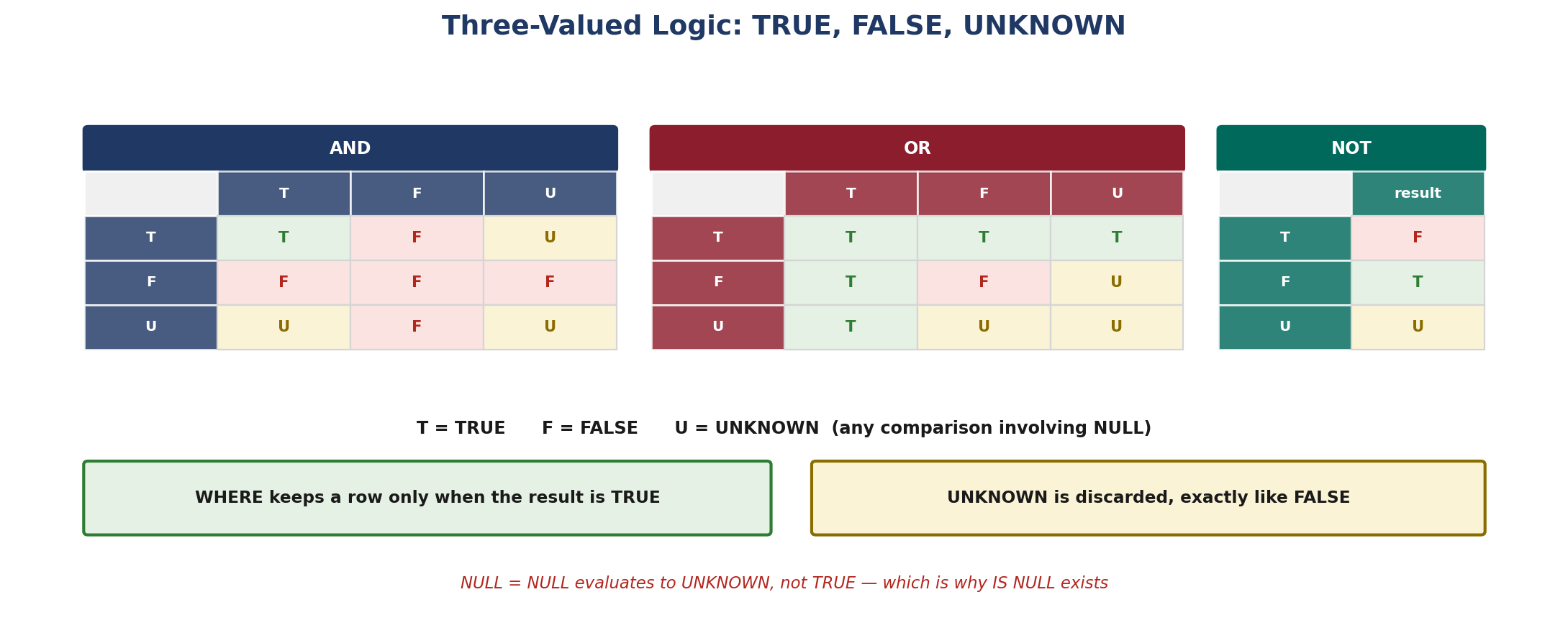
Three-valued logic: TRUE, FALSE, UNKNOWN

Figure 5.1 — How AND, OR, and NOT behave with UNKNOWN.

WHERE keeps a row only when the condition is TRUE. UNKNOWN is discarded exactly as FALSE is, which is why rows containing NULL quietly disappear from results that seem like they should include them.

SELECT 1 = 1          AS Comparison1,
       1 = 2          AS Comparison2
WHERE  1 = 1;

SELECT EmployeeID, Email
FROM   HR.Employees
WHERE  Email = NULL;

SELECT EmployeeID, Email
FROM   HR.Employees
WHERE  Email IS NULL;

The second query returns nothing at all. Only the third finds rows with a missing email.

5.2 IS NULL and IS NOT NULL

SELECT EmployeeID, FirstName, Email
FROM   HR.Employees
WHERE  Email IS NULL;

SELECT EmployeeID, FirstName, Email
FROM   HR.Employees
WHERE  Email IS NOT NULL;

SELECT EmployeeID, FirstName, ManagerID, Email
FROM   HR.Employees
WHERE  ManagerID IS NULL
   AND Email IS NOT NULL;

SELECT COUNT(*)                                                  AS TotalRows,
       SUM(CASE WHEN Email IS NULL THEN 1 ELSE 0 END)            AS MissingEmail,
       SUM(CASE WHEN ManagerID IS NULL THEN 1 ELSE 0 END)        AS MissingManager
FROM   HR.Employees;

The last query profiles how complete each column is — a standard first step on any new dataset.

5.3 NULL, Zero, and Empty String

These three look similar in a result grid and behave completely differently. Zero is a known quantity. An empty string is a known string of length zero. NULL is the absence of any value at all.

	NULL	0	'' (empty string)
Meaning	Unknown or not applicable	A known value of zero	A known string with no characters
Storage	Marked absent	Numeric zero	Zero-length string
Equality test	IS NULL only	`= 0` works	`= ''` works
LEN() result	NULL	1	0
Counted by COUNT(col)	No	Yes	Yes
Included in SUM	Ignored	Yes	N/A

SELECT LEN(NULL)               AS LengthOfNull,
       LEN('')                 AS LengthOfEmpty,
       LEN(' ')                AS LengthOfSpace,
       NULL + 100              AS NullArithmetic,
       0 + 100                 AS ZeroArithmetic,
       DATALENGTH(NULL)        AS DataLengthNull,
       DATALENGTH('')          AS DataLengthEmpty;

LEN(NULL) is NULL, LEN('') is 0, and adding anything to NULL yields NULL.

SELECT EmployeeID, Email
FROM   HR.Employees
WHERE  Email IS NULL
    OR LTRIM(RTRIM(Email)) = '';

Datasets loaded from files frequently contain both, so a completeness check should test for each.

5.4 NULL in Aggregates

Aggregate functions ignore NULL. This is usually helpful and occasionally misleading, because AVG divides by the count of non-NULL values rather than the number of rows.

SELECT COUNT(*)                   AS AllRows,
       COUNT(Salary)              AS RowsWithSalary,
       COUNT(Bonus)               AS RowsWithBonus,
       SUM(Bonus)                 AS TotalBonus,
       AVG(Bonus)                 AS AverageBonusNonNullOnly,
       AVG(ISNULL(Bonus, 0))      AS AverageBonusTreatingNullAsZero
FROM   HR.Employees;

The last two columns differ whenever any bonus is NULL, and both can be the correct answer depending on the question.

COUNT(*): counts rows, including rows that are entirely NULL.
COUNT(column): counts non-NULL values in that column only.
SUM, AVG, MIN, MAX: skip NULLs entirely rather than treating them as zero.
AVG: divides by the non-NULL count — decide explicitly whether missing should mean zero.

5.5 NULL in GROUP BY, DISTINCT, and Constraints

Grouping and DISTINCT treat all NULLs as equal to each other, even though a comparison between two NULLs returns UNKNOWN. This inconsistency is deliberate and defined by the standard.

SELECT   DepartmentID, COUNT(*) AS HeadCount
FROM     HR.Employees
GROUP BY DepartmentID;

SELECT DISTINCT DepartmentID
FROM   HR.Employees;

Both return a single row or group for NULL, collecting every unassigned employee together.

A UNIQUE constraint follows the same rule in SQL Server: it permits one NULL and rejects a second. A PRIMARY KEY forbids NULL entirely.

5.6 The NOT IN Trap

This is the most damaging NULL behaviour in practice. If the list or subquery behind NOT IN contains even one NULL, the entire predicate evaluates to UNKNOWN for every row, and the query returns nothing.

SELECT EmployeeID, FirstName
FROM   HR.Employees
WHERE  DepartmentID NOT IN
(
    SELECT DepartmentID
    FROM   HR.Departments
);

Returns zero rows if any DepartmentID in HR.Departments is NULL, even though rows clearly qualify.

SELECT EmployeeID, FirstName
FROM   HR.Employees
WHERE  DepartmentID NOT IN
(
    SELECT DepartmentID
    FROM   HR.Departments
    WHERE  DepartmentID IS NOT NULL
);

SELECT e.EmployeeID, e.FirstName
FROM   HR.Employees AS e
WHERE  NOT EXISTS
(
    SELECT 1
    FROM   HR.Departments AS d
    WHERE  d.DepartmentID = e.DepartmentID
);

Either filter the NULLs out, or use NOT EXISTS — which is immune to the problem and usually faster.

5.7 COALESCE

COALESCE returns the first non-NULL value from a list of expressions. It is ANSI standard, accepts any number of arguments, and is the general-purpose tool for supplying fallbacks.

SELECT EmployeeID,
       COALESCE(Email, 'no email on file')                     AS ContactEmail,
       COALESCE(ManagerID, EmployeeID)                         AS EffectiveManagerID,
       COALESCE(Bonus, 0)                                      AS BonusOrZero,
       COALESCE(MobilePhone, OfficePhone, HomePhone, 'none')   AS BestContactNumber
FROM   HR.Employees;

The final column walks three columns in priority order and falls back to a literal.

SELECT EmployeeID,
       Salary,
       Bonus,
       Salary + COALESCE(Bonus, 0)   AS TotalCompensation,
       Salary + Bonus                AS TotalCompensationBroken
FROM   HR.Employees;

Without COALESCE, every employee with no bonus shows NULL total compensation instead of their salary.

Function	Behaviour	Notes
COALESCE(a, b, ...)	Returns the first non-NULL argument	ANSI standard, any number of arguments
ISNULL(a, b)	Returns b if a is NULL	T-SQL only, exactly two arguments
NULLIF(a, b)	Returns NULL if a equals b, else a	Useful for guarding division by zero
IIF(cond, a, b)	Shorthand conditional	T-SQL only; CASE is the portable form
TRY_CAST / TRY_CONVERT	Returns NULL instead of failing	Safe conversion of dirty data

COALESCE and ISNULL differ in more than argument count. ISNULL takes the data type of its first argument, which can silently truncate the replacement value; COALESCE applies standard type precedence across all arguments.

SELECT ISNULL(CAST(NULL AS VARCHAR(3)), 'Chennai')    AS IsnullTruncated,
       COALESCE(CAST(NULL AS VARCHAR(3)), 'Chennai')  AS CoalesceFull;

ISNULL returns 'Che' because it adopts VARCHAR(3) from the first argument. COALESCE returns 'Chennai'.

SELECT EmployeeID,
       Salary,
       TargetSalary,
       Salary / NULLIF(TargetSalary, 0)   AS AchievementRatio
FROM   HR.Employees;

NULLIF converts a zero divisor into NULL, so the row returns NULL instead of raising a divide-by-zero error.

SELECT EmployeeID,
       HireDateText,
       TRY_CAST(HireDateText AS DATE)   AS ParsedHireDate
FROM   Staging.EmployeeImport
WHERE  TRY_CAST(HireDateText AS DATE) IS NULL;

TRY_CAST returns NULL for unparseable values, which turns a failing load into a reviewable exception list.

5.9 Deciding How to Handle Missing Values

Replacing NULL is a modelling decision, not a formatting one. Substituting zero changes averages; substituting a placeholder string change counts of distinct values. The right choice depends on what the missing value means.

Situation	Reasonable handling
Bonus not yet awarded	`COALESCE(Bonus, 0)` — no bonus genuinely means zero
Salary not recorded	Leave NULL — zero would corrupt the average
Email not supplied	COALESCE for display only; keep NULL in the data
Top of a reporting hierarchy	`ManagerID IS NULL` is meaningful — do not replace it
Optional end date on a project	NULL means still running — preserve it

SELECT      e.EmployeeID,
            CONCAT(e.FirstName, ' ', e.LastName)      AS FullName,
            COALESCE(e.Email, 'not provided')         AS ContactEmail,
            e.Salary,
            COALESCE(e.Bonus, 0)                      AS BonusApplied,
            e.Salary + COALESCE(e.Bonus, 0)           AS TotalCompensation,
            CASE WHEN e.ManagerID IS NULL
                 THEN 'Top of hierarchy'
                 ELSE CAST(e.ManagerID AS VARCHAR(10))
            END                                       AS ReportsTo
FROM        HR.Employees AS e
WHERE       e.IsActive = 1
ORDER BY    TotalCompensation DESC;

Display NULLs are replaced, meaningful NULLs are preserved and labelled, and the arithmetic is protected.

Best Practice: Never compare NULL using = NULL, and decide explicitly how missing values should be handled.

Hands-On: Find all rows containing NULL values in the provided dataset. Compare NULL behaviour against zero and empty string using LEN, DATALENGTH, arithmetic, and COUNT. Write queries using IS NULL and IS NOT NULL, then replace displayed NULLs with COALESCE and ISNULL. Demonstrate the NOT IN trap and fix it two ways. Finally, show a case where replacing NULL with zero changes an average, and justify which result is correct.

Phase 5 – SQL Functions & Aggregations

Phase 5 Overview

Every script in this phase is directly runnable. Scripts assume SQL Server and an employees/orders schema, defined at the start of Module 1.

#	Subtopic	Learning Outcome
1	Built-in SQL Functions	String, numeric, date, conversion, and NULL-handling functions; avoiding functions on filtered/indexed columns
2	Aggregate Functions	COUNT, SUM, AVG, MIN, MAX and how each one treats NULL
3	GROUP BY	Grouping by one and multiple columns; the rule that ties SELECT columns to GROUP BY
4	HAVING	Filtering groups vs. filtering rows; combining WHERE, GROUP BY, and HAVING correctly
5	Conditional Logic — CASE	Labelling ranges, sorting, and conditional aggregation with CASE

Module 1: Built-in SQL Functions

1.1 Sample Schema

The examples below use two tables. Create them once and reuse them for every module in this phase.

CREATE TABLE employees (
    emp_id      INT PRIMARY KEY,
    first_name  VARCHAR(50),
    last_name   VARCHAR(50),
    department  VARCHAR(50),
    salary      DECIMAL(10,2),
    hire_date   DATE,
    bonus       DECIMAL(10,2)
);

INSERT INTO employees VALUES
(1, 'Asha',   'Kumar',  'Sales',   52000, '2019-03-14', 2000),
(2, 'Ravi',   'Menon',  'Sales',   61000, '2020-07-01', NULL),
(3, 'Priya',  'Nair',   'IT',      75000, '2018-11-23', 5000),
(4, 'John',   'Mathew', 'IT',      82000, '2021-01-10', NULL),
(5, 'Divya',  'Suresh', 'HR',      45000, '2022-06-15', 1000),
(6, 'Karan',  'Shah',   'HR',      47000, '2017-09-05', NULL),
(7, 'Meera',  'Iyer',   'IT',      91000, '2015-02-20', 7000),
(8, 'Arjun',  'Pillai', 'Sales',   58000, '2023-04-11', 1500),
(9, 'Nisha',  'Rao',    'Finance', 68000, '2019-12-01', NULL),
(10,'Vikram', 'Desai',  'Finance', 72000, '2020-08-19', 3000);

bonus is deliberately left NULL for four employees — this drives the NULL discussion in Module 2.

1.2 String Functions

Function	Purpose	Example
UPPER / LOWER	Change case	`UPPER(first_name)`
CONCAT	Join strings	`CONCAT(first_name,' ',last_name)`
LENGTH / LEN	Character count	`LENGTH(last_name)`
SUBSTRING	Extract part of a string	`SUBSTRING(last_name,1,3)`

SELECT
    UPPER(first_name)                    AS name_upper,
    LOWER(department)                    AS dept_lower,
    CONCAT(first_name, ' ', last_name)   AS full_name,
    LENGTH(last_name)                    AS name_length,
    SUBSTRING(last_name, 1, 3)           AS name_prefix
FROM employees;

1.3 Numeric Functions

SELECT
    emp_id,
    salary,
    ROUND(salary * 0.10, 2)    AS ten_pct_raise,
    CEIL(salary / 1000.0)      AS salary_in_k_rounded_up,
    FLOOR(salary / 1000.0)     AS salary_in_k_rounded_down,
    ABS(-500)                  AS abs_example
FROM employees;

ROUND, CEIL/CEILING, FLOOR, and ABS cover the numeric adjustments used most often in reporting.

1.4 Date Functions

SELECT
    emp_id,
    hire_date,
    CURRENT_DATE                              AS today,
    DATEDIFF(CURRENT_DATE, hire_date)         AS days_employed,
    YEAR(hire_date)                           AS hire_year,
    DATE_ADD(hire_date, INTERVAL 5 YEAR)      AS five_year_mark
FROM employees;

Shown in MySQL syntax. PostgreSQL: CURRENT_DATE - hire_date, EXTRACT(YEAR FROM hire_date), hire_date + INTERVAL '5 years'.

1.5 Conversion Functions

SELECT
    CAST(salary AS VARCHAR(20))       AS salary_as_text,
    CONVERT(salary, DECIMAL(10,0))    AS salary_no_decimals
FROM employees;

CAST is the ANSI-standard form; CONVERT is T-SQL specific and adds style codes for dates.

1.6 NULL-Handling Functions

SELECT
    emp_id,
    bonus,
    COALESCE(bonus, 0)               AS bonus_safe,
    IFNULL(bonus, 0)                 AS bonus_safe_mysql,
    salary + COALESCE(bonus, 0)      AS total_comp
FROM employees;

COALESCE is ANSI-standard and accepts any number of arguments; IFNULL and ISNULL are engine-specific two-argument versions.

1.7 Functions and Index Usage

Wrapping a filtered or indexed column in a function usually prevents the optimizer from using an index on that column, because the engine would have to evaluate the function for every row before it can compare. The fix is to transform the constant on the other side of the comparison instead of the column.

-- Not index-friendly: function wraps the filtered column
SELECT * FROM employees WHERE YEAR(hire_date) = 2020;

-- Index-friendly: hire_date itself is compared directly
SELECT * FROM employees
WHERE hire_date >= '2020-01-01' AND hire_date < '2021-01-01';

Both queries return the same rows; only the second can use an index on hire_date efficiently.

Best Practice: Reserve functions for the SELECT list and for values you are not filtering on.

Hands-On: Using the employees table, write one query per function category (string, numeric, date, conversion, NULL-handling). Then take the YEAR(hire_date) = 2020 example, rewrite it as a date range, and compare the two execution plans if your environment supports SHOWPLAN or EXPLAIN.

Module 2: Aggregate Functions

2.1 The Five Core Aggregates

Function	Description
COUNT	Number of rows, or number of non-NULL values in a column
SUM	Total of a numeric column, ignoring NULLs
AVG	Mean of a numeric column, ignoring NULLs
MIN / MAX	Smallest / largest non-NULL value

SELECT
    COUNT(*)       AS total_rows,
    COUNT(bonus)   AS employees_with_bonus,
    SUM(salary)    AS total_salary,
    AVG(salary)    AS avg_salary,
    MIN(salary)    AS min_salary,
    MAX(salary)    AS max_salary,
    SUM(bonus)     AS total_bonus,
    AVG(bonus)     AS avg_bonus
FROM employees;

2.2 How Aggregates Handle NULL

The employees table has four NULL values in bonus out of ten rows. Repeating the aggregate query and reading the results against this table shows exactly what NULL does to each function.

Function	Behaviour with NULL	Result on bonus (4 NULLs of 10 rows)
COUNT(bonus)	Ignores NULLs entirely	Counts only the 6 rows with a bonus, not 10
`COUNT(*)`	Counts rows regardless of NULLs	Always 10
SUM(bonus)	NULLs contribute nothing (not treated as 0)	Sum of only the 6 non-NULL bonuses
AVG(bonus)	Divides by the count of non-NULL values	SUM(bonus) / 6, not / 10
MIN / MAX(bonus)	NULLs are skipped when comparing	True min/max among non-NULL values

2.3 NULL Is Not Zero

Wrapping bonus in COALESCE before averaging changes the denominator, which changes the answer.

SELECT
    AVG(bonus)                  AS avg_ignoring_nulls,
    AVG(COALESCE(bonus, 0))     AS avg_treating_null_as_zero
FROM employees;

Best Practice: Before trusting an AVG, check whether the column actually contains NULLs.

Hands-On: Run the aggregate query on employees as written, then again with bonus wrapped in COALESCE(bonus, 0). Write down both AVG values and explain in one sentence why they differ.

Module 3: GROUP BY

3.1 Grouping by One Column

SELECT
    department,
    COUNT(*)      AS headcount,
    AVG(salary)   AS avg_salary,
    SUM(salary)   AS total_salary
FROM employees
GROUP BY department
ORDER BY department;

Expected output:

department	headcount	avg_salary	total_salary
Finance	2	70000.00	140000.00
HR	2	46000.00	92000.00
IT	3	82666.67	248000.00
Sales	3	57000.00	171000.00

3.2 Grouping by Multiple Columns

SELECT
    department,
    YEAR(hire_date)   AS hire_year,
    COUNT(*)          AS headcount,
    AVG(salary)       AS avg_salary
FROM employees
GROUP BY department, YEAR(hire_date)
ORDER BY department, hire_year;

Each unique (department, hire_year) pair becomes its own summary row — a finer grouping than department alone.

3.3 The Rule: Group or Aggregate, No Exceptions

-- Invalid: first_name is neither grouped nor aggregated
SELECT department, first_name, AVG(salary)
FROM employees
GROUP BY department;

-- Fixed: drop the ungrouped column, or add it to GROUP BY
SELECT department, AVG(salary)
FROM employees
GROUP BY department;

Best Practice: Decide the grain of the report first — one row per department, or per department and year — then let that decide the GROUP BY list.

Hands-On: Reproduce the department-level GROUP BY above and check it against the expected output table. Then write a second query grouped by department and hire year, and predict how many rows it returns before running it.

Module 4: HAVING

4.1 WHERE Filters Rows, HAVING Filters Groups

Aspect	WHERE	HAVING
Runs relative to GROUP BY	Before grouping	After grouping
Filters	Individual rows	Group summaries
Can reference aggregates?	No	Yes
Typical use	`department = 'IT'`	`AVG(salary) > 60000`

4.2 Using WHERE, GROUP BY, and HAVING Together

SELECT
    department,
    COUNT(*)      AS headcount,
    AVG(salary)   AS avg_salary
FROM employees
WHERE hire_date >= '2018-01-01'
GROUP BY department
HAVING AVG(salary) > 55000
ORDER BY avg_salary DESC;

Order of execution: FROM → WHERE → GROUP BY → HAVING → SELECT → ORDER BY.

4.3 Rewriting Incorrect Examples

Incorrect — an aggregate referenced in WHERE:

-- Fails: AVG(salary) does not exist yet when WHERE runs
SELECT department, AVG(salary)
FROM employees
WHERE AVG(salary) > 60000
GROUP BY department;

Fix — move the condition to HAVING:

SELECT department, AVG(salary)
FROM employees
GROUP BY department
HAVING AVG(salary) > 60000;

Incorrect — a row-level condition placed in HAVING:

-- Works, but wasteful: filters department after grouping
SELECT department, COUNT(*)
FROM employees
GROUP BY department
HAVING department = 'IT';

Fix — move the condition to WHERE so fewer rows reach GROUP BY:

SELECT department, COUNT(*)
FROM employees
WHERE department = 'IT'
GROUP BY department;

Best Practice: Ask what the condition is actually about.

Hands-On: Write the combined WHERE + GROUP BY + HAVING query above from scratch, then take both incorrect examples and rewrite them yourself before checking against the fixes.

Module 5: Conditional Logic — CASE

5.1 CASE to Label Numeric Ranges

SELECT
    emp_id,
    salary,
    CASE
        WHEN salary < 50000                  THEN 'Low'
        WHEN salary BETWEEN 50000 AND 75000  THEN 'Medium'
        WHEN salary > 75000                  THEN 'High'
    END AS salary_band
FROM employees;

5.2 CASE Inside ORDER BY

-- Custom sort order: High first, then Medium, then Low
SELECT emp_id, salary
FROM employees
ORDER BY
    CASE
        WHEN salary > 75000                  THEN 1
        WHEN salary BETWEEN 50000 AND 75000  THEN 2
        ELSE 3
    END;

5.3 CASE for Conditional Aggregation

-- Count employees per band, pivoted into columns
SELECT
    department,
    SUM(CASE WHEN salary < 50000                 THEN 1 ELSE 0 END) AS low_count,
    SUM(CASE WHEN salary BETWEEN 50000 AND 75000 THEN 1 ELSE 0 END) AS medium_count,
    SUM(CASE WHEN salary > 75000                 THEN 1 ELSE 0 END) AS high_count
FROM employees
GROUP BY department
ORDER BY department;

5.4 Keeping CASE Readable

Nest one CASE inside another and the logic becomes hard to audit at a glance. Flattening the conditions into additional top-level WHEN branches produces the same result without the nesting.

Nested — hard to read:

SELECT emp_id,
  CASE
    WHEN department = 'IT' THEN
      CASE WHEN salary > 80000 THEN 'Senior IT' ELSE 'Junior IT' END
    ELSE 'Other'
  END AS role_band
FROM employees;

Flattened — same result, no nesting:

SELECT emp_id,
  CASE
    WHEN department = 'IT' AND salary > 80000 THEN 'Senior IT'
    WHEN department = 'IT'                    THEN 'Junior IT'
    ELSE 'Other'
  END AS role_band
FROM employees;

Best Practice: Put each WHEN on its own line, keep CASE expressions flat rather than nested, and always include an ELSE unless a NULL fallback is genuinely intended.

Hands-On: Write the Low/Medium/High CASE query, then reuse the same condition inside SUM(CASE ...) to build the conditional aggregation. Finally, take one nested CASE example of your own and flatten it.

Phase 6 Overview

Every script in this phase is directly runnable. Scripts assume SQL Server and the departments / employees / customers / orders / products / order_items schema defined at the start of Module 1.

#	Subtopic	Learning Outcome
1	Introduction to Joins	Why joins are needed, explicit JOIN syntax, meaningful aliases, and an INNER JOIN with an explicit column list
2	Types of Joins	INNER, LEFT, RIGHT, FULL OUTER, CROSS, and SELF JOIN — predicting rows before running each one
3	Advanced Join Scenarios	Joining three, four, and five tables; verifying row counts; troubleshooting duplicates and missing rows
4	Set Operators	UNION, UNION ALL, INTERSECT, and EXCEPT; column-count and data-type compatibility

Module 1: Introduction to Joins

1.1 Sample Schema

The examples in this phase use six related tables. Create them once and reuse them for every module.

CREATE TABLE departments (
    department_id   INT PRIMARY KEY,
    department_name VARCHAR(50)
);

CREATE TABLE employees (
    emp_id        INT PRIMARY KEY,
    first_name    VARCHAR(50),
    last_name     VARCHAR(50),
    department_id INT,        -- FK -> departments.department_id (NULL = unassigned)
    manager_id    INT,        -- FK -> employees.emp_id (self-reference)
    salary        DECIMAL(10,2),
    city          VARCHAR(50)
);

CREATE TABLE customers (
    customer_id   INT PRIMARY KEY,
    customer_name VARCHAR(60),
    city          VARCHAR(50)
);

CREATE TABLE orders (
    order_id    INT PRIMARY KEY,
    customer_id INT,          -- FK -> customers.customer_id
    emp_id      INT,          -- FK -> employees.emp_id (NULL = unassigned rep)
    order_date  DATE,
    amount      DECIMAL(10,2)
);

CREATE TABLE products (
    product_id   INT PRIMARY KEY,
    product_name VARCHAR(60),
    category     VARCHAR(30),
    unit_price   DECIMAL(10,2)
);

CREATE TABLE order_items (
    order_item_id INT PRIMARY KEY,
    order_id      INT,        -- FK -> orders.order_id
    product_id    INT,        -- FK -> products.product_id
    quantity      INT
);

INSERT INTO departments VALUES
(1,'Sales'), (2,'IT'), (3,'HR'), (4,'Finance'), (5,'Marketing');

INSERT INTO employees VALUES
(1, 'Asha',   'Kumar',   1,    NULL, 52000, 'Chennai'),
(2, 'Ravi',   'Menon',   1,    1,    61000, 'Chennai'),
(3, 'Priya',  'Nair',    2,    NULL, 75000, 'Bengaluru'),
(4, 'John',   'Mathew',  2,    3,    82000, 'Bengaluru'),
(5, 'Divya',  'Suresh',  3,    NULL, 45000, 'Mumbai'),
(6, 'Karan',  'Shah',    3,    5,    47000, 'Mumbai'),
(7, 'Meera',  'Iyer',    2,    3,    91000, 'Bengaluru'),
(8, 'Arjun',  'Pillai',  1,    1,    58000, 'Chennai'),
(9, 'Nisha',  'Rao',     4,    NULL, 68000, 'Delhi'),
(10,'Vikram', 'Desai',   4,    9,    72000, 'Delhi'),
(11,'Rohan',  'Kapoor',  NULL, NULL, 40000, 'Pune');

INSERT INTO customers VALUES
(1, 'Meridian Textiles',   'Chennai'),
(2, 'BlueWave Retail',     'Mumbai'),
(3, 'Northstar Logistics', 'Delhi'),
(4, 'Orchid Foods',        'Bengaluru'),
(5, 'Copper Hardware',     'Coimbatore'),
(6, 'Skyline Traders',     'Chennai');

INSERT INTO orders VALUES
(101, 1, 2,    '2024-01-05', 12000),
(102, 1, 2,    '2024-02-10', 8000),
(103, 2, 6,    '2024-01-20', 15500),
(104, 4, 8,    '2024-03-01', 9500),
(105, 3, 10,   '2024-03-15', 21000),
(106, 2, 6,    '2024-04-02', 17600),
(107, 5, 8,    '2024-04-20', 6000),
(108, 1, NULL, '2024-05-01', 4300);

INSERT INTO products VALUES
(201,'Steel Bracket','Hardware',150),
(202,'Wireless Mouse','Electronics',899),
(203,'Organic Almonds','Grocery',450),
(204,'Cotton Fabric Roll','Textiles',1200),
(205,'LED Desk Lamp','Electronics',650);

INSERT INTO order_items VALUES
(1, 101, 204, 10), (2, 101, 201, 5), (3, 102, 202, 3),
(4, 103, 203, 20), (5, 104, 203, 15), (6, 105, 204, 8),
(7, 106, 205, 4),  (8, 107, 201, 12),(9, 108, 202, 2);

Department 5 (Marketing) has no employees, employee 11 (Rohan) has no department, order 108 has no assigned employee, and customer 6 (Skyline) has never ordered — each gap is used deliberately later in this phase.

1.2 Explicit JOIN Syntax and Meaningful Aliases

Older code sometimes lists tables separated by commas and puts the join condition in WHERE. That still works, but it hides the join logic among ordinary filters and makes it easy to forget a condition by accident. Explicit JOIN syntax states the join type and its condition together, and a short alias keeps every column reference unambiguous.

-- Implicit style: works, but easy to misread as two unrelated filters
SELECT employees.first_name, departments.department_name
FROM employees, departments
WHERE employees.department_id = departments.department_id;

-- Explicit style: the join type and condition are stated together
SELECT e.first_name, d.department_name
FROM employees AS e
INNER JOIN departments AS d
    ON e.department_id = d.department_id;

Both return the same rows here, but only the explicit form makes the join condition impossible to lose track of as a query grows.

1.3 Writing an INNER JOIN with an Explicit Column List

SELECT * is convenient while exploring, but a finished query should name exactly the columns it needs — it documents intent and survives schema changes better.

SELECT
    e.emp_id,
    e.first_name,
    e.last_name,
    d.department_name
FROM employees AS e
INNER JOIN departments AS d
    ON e.department_id = d.department_id
ORDER BY e.emp_id;

Returns 10 rows. Rohan Kapoor (department_id is NULL) has no matching department row, so INNER JOIN drops him.

Best Practice: Always write JOIN ... ON with meaningful table aliases instead of listing tables with commas and joining in WHERE.

Hands-On: Using employees and departments, write an INNER JOIN that returns emp_id, first_name, last_name, and department_name, ordered by emp_id. Predict the row count before running it, then confirm which employee is missing and why.

Module 2: Types of Joins

2.1 INNER JOIN — Only Matched Rows

SELECT e.emp_id, e.first_name, d.department_name
FROM employees AS e
INNER JOIN departments AS d
    ON e.department_id = d.department_id
ORDER BY e.emp_id;

10 rows. Only employees with a valid department_id survive; Rohan is dropped.

2.2 LEFT (OUTER) JOIN — Every Row on the Left

SELECT e.emp_id, e.first_name, d.department_name
FROM employees AS e
LEFT JOIN departments AS d
    ON e.department_id = d.department_id
ORDER BY e.emp_id;

11 rows. Every employee appears; Rohan's department_name comes back NULL instead of disappearing.

2.3 RIGHT (OUTER) JOIN — Every Row on the Right

SELECT d.department_name, e.emp_id, e.first_name
FROM employees AS e
RIGHT JOIN departments AS d
    ON e.department_id = d.department_id
ORDER BY d.department_id;

11 rows. Every department appears; Marketing (department_id 5) has no employees, so emp_id and first_name come back NULL for it.

2.4 FULL OUTER JOIN — Every Row on Either Side

SELECT e.emp_id, e.first_name, d.department_name
FROM employees AS e
FULL OUTER JOIN departments AS d
    ON e.department_id = d.department_id
ORDER BY d.department_id, e.emp_id;

12 rows: all 10 matched pairs, plus Rohan (NULL department) and Marketing (NULL employee). MySQL has no FULL OUTER JOIN keyword — emulate it with a LEFT JOIN UNION a RIGHT JOIN.

2.5 CROSS JOIN — Every Combination

SELECT d.department_name, p.product_name
FROM departments AS d
CROSS JOIN products AS p
ORDER BY d.department_name, p.product_name;

25 rows (5 departments x 5 products) — every possible pairing, with no ON clause at all. Useful for building a coverage matrix on purpose; almost never wanted by accident.

2.6 SELF JOIN — A Table Joined to Itself

employees.manager_id points back to employees.emp_id. Joining the table to itself, once as the employee and once as the manager, resolves that relationship into readable pairs.

SELECT
    m.first_name AS manager_first_name,
    e.first_name AS employee_first_name
FROM employees AS e
INNER JOIN employees AS m
    ON e.manager_id = m.emp_id
ORDER BY manager_first_name;

6 rows — one per employee who has a manager assigned. Asha, Priya, Divya, Nisha (top-level managers) and Rohan (no manager) are excluded because nothing joins to them on this condition.

2.7 Predict, Then Verify

Before running any of the queries above, write down the predicted row count and the reasoning. Then run the query and compare.

Join Type	Predicted Rows	Why
INNER JOIN	10	Only employees with a real department_id match
LEFT JOIN	11	All employees; Rohan gets a NULL department
RIGHT JOIN	11	All departments; Marketing gets a NULL employee
FULL OUTER JOIN	12	All matches, plus Rohan and Marketing both unmatched
CROSS JOIN	25	5 departments x 5 products, no condition to filter it
SELF JOIN	6	Only employees who have a non-NULL manager_id

Best Practice: Pick the join type by deciding what should happen to unmatched rows before writing the query, not by trial and error afterward.

Hands-On: Run all six join queries above against the schema from Module 1. For each one, write your predicted row count first, then compare it to the actual count and explain any difference in one sentence.

Module 3: Advanced Join Scenarios

3.1 Joining Three Tables

SELECT
    o.order_id,
    c.customer_name,
    e.first_name AS handled_by,
    o.amount
FROM orders AS o
INNER JOIN customers AS c ON o.customer_id = c.customer_id
INNER JOIN employees AS e ON o.emp_id      = e.emp_id
ORDER BY o.order_id;

7 rows. Order 108 is dropped: its emp_id is NULL, so it has no match in employees.

3.2 Joining Four Tables

SELECT
    o.order_id,
    c.customer_name,
    e.first_name AS handled_by,
    d.department_name,
    o.amount
FROM orders AS o
INNER JOIN customers   AS c ON o.customer_id   = c.customer_id
INNER JOIN employees   AS e ON o.emp_id        = e.emp_id
INNER JOIN departments AS d ON e.department_id = d.department_id
ORDER BY o.order_id;

Still 7 rows. Every employee who has handled an order also has a valid department, so adding departments does not change the count — a useful check in itself.

3.3 Joining Five Tables

SELECT
    oi.order_item_id,
    o.order_id,
    c.customer_name,
    e.first_name AS handled_by,
    d.department_name,
    oi.quantity
FROM order_items AS oi
INNER JOIN orders      AS o ON oi.order_id     = o.order_id
INNER JOIN customers   AS c ON o.customer_id   = c.customer_id
INNER JOIN employees   AS e ON o.emp_id        = e.emp_id
INNER JOIN departments AS d ON e.department_id = d.department_id
ORDER BY oi.order_item_id;

8 rows, not 9. order_item_id 9 belongs to order 108, which has no employee — the same gap from Module 3.1 removes one more row once order_items is added.

3.4 Verifying Row Counts at Every Step

Build a multi-table join incrementally and check COUNT(*) after each JOIN is added, rather than writing the whole chain first and hoping. A count that jumps up unexpectedly signals a join matching more than one row per row on one side; a count that drops signals rows without a valid match on the other side.

SELECT COUNT(*) FROM order_items;                                  -- 9

SELECT COUNT(*)
FROM order_items AS oi
INNER JOIN orders AS o ON oi.order_id = o.order_id;                -- 9, unchanged: every item has a valid order

SELECT COUNT(*)
FROM order_items AS oi
INNER JOIN orders    AS o ON oi.order_id = o.order_id
INNER JOIN employees AS e ON o.emp_id    = e.emp_id;               -- 8, dropped: order 108 has no employee

3.5 Troubleshooting Duplicates, Missing Rows, and Cartesian Products

A Cartesian product — a missing or forgotten join condition:

-- Cartesian product: the join condition was left out entirely
SELECT o.order_id, c.customer_name
FROM orders AS o, customers AS c;
-- 8 orders x 6 customers = 48 rows

Fix:

SELECT o.order_id, c.customer_name
FROM orders AS o
INNER JOIN customers AS c ON o.customer_id = c.customer_id;
-- 8 rows: one per order

Duplicate rows — a join fans out before an aggregate is taken:

-- order_items has two rows for order 101, so amount is repeated
SELECT o.order_id, o.amount, oi.order_item_id
FROM orders AS o
INNER JOIN order_items AS oi ON o.order_id = oi.order_id
WHERE o.order_id = 101;
-- 2 rows, both showing amount = 12000 — summing amount here would double it

Fix — aggregate at the grain you actually need before or after the join:

SELECT o.order_id, o.amount
FROM orders AS o
WHERE o.order_id = 101;
-- 1 row: the order amount itself is not affected by how many items it has

Missing rows — the wrong join type silently drops data:

-- INNER JOIN drops customers who have never placed an order
SELECT c.customer_id, c.customer_name, COUNT(o.order_id) AS order_count
FROM customers AS c
INNER JOIN orders AS o ON c.customer_id = o.customer_id
GROUP BY c.customer_id, c.customer_name;
-- Skyline Traders never appears at all

Fix — LEFT JOIN keeps every customer, including those with zero orders:

SELECT c.customer_id, c.customer_name, COUNT(o.order_id) AS order_count
FROM customers AS c
LEFT JOIN orders AS o ON c.customer_id = o.customer_id
GROUP BY c.customer_id, c.customer_name;
-- Skyline Traders now appears with order_count = 0

COUNT(o.order_id) counts the column, not COUNT(*) — so a customer with no matching order (a NULL order_id) correctly counts as 0, not 1.

Best Practice: Add one table and one JOIN at a time, checking COUNT(*) after each addition, instead of writing a five-table join in one pass.

Hands-On: Build the five-table join in Module 3.3 one JOIN at a time, recording the row count after each addition. Then take the three broken examples in 3.5, predict what each one will return before running it, and confirm.

Module 4: Set Operators

4.1 UNION vs. UNION ALL

customers has 6 rows (two of them in Chennai); employees has 11 rows. UNION removes duplicate rows from the combined set; UNION ALL keeps every row from both sides.

SELECT city FROM customers
UNION
SELECT city FROM employees;

6 distinct rows: Chennai, Mumbai, Delhi, Bengaluru, Coimbatore, Pune — duplicates across and within both lists are collapsed.

SELECT city FROM customers
UNION ALL
SELECT city FROM employees;

17 rows: 6 from customers plus 11 from employees, with every duplicate — including Chennai appearing three times — kept.

4.2 INTERSECT

INTERSECT returns only the rows that appear in both result sets.

SELECT city FROM customers
INTERSECT
SELECT city FROM employees;

4 rows: Chennai, Mumbai, Delhi, Bengaluru — the cities with both a customer and an employee.

4.3 EXCEPT

EXCEPT returns rows from the first result set that do not appear in the second. Order matters — swapping the two queries changes the answer.

SELECT city FROM customers
EXCEPT
SELECT city FROM employees;

1 row: Coimbatore — a customer city with no employee in it.

SELECT city FROM employees
EXCEPT
SELECT city FROM customers;

1 row: Pune — an employee city with no customer in it. This is the reverse comparison, not the same query re-run.

4.4 Column and Type Compatibility

-- Fails: the left side has 2 columns, the right side has 1
SELECT customer_id, customer_name FROM customers
UNION
SELECT emp_id FROM employees;

Fix — match the column count and give both sides compatible types:

SELECT customer_id AS person_id, customer_name AS person_name FROM customers
UNION
SELECT emp_id, first_name FROM employees;

The result's column names come from the first SELECT — person_id and person_name — regardless of what the second query calls them.

Best Practice: Default to UNION ALL unless duplicates genuinely need removing — it skips the extra sort/dedupe step and is cheaper to run.

Hands-On: Run all four set operators on the customers and employees city lists above, and record the row count each one returns. Then break the column-compatibility rule on purpose, read the error, and fix it.

Phase 7 Overview

Every script in this phase is directly runnable. Scripts assume SQL Server and the departments / employees / customers / orders / products / order_items schema introduced in Phase 6.

#	Subtopic	Learning Outcome
1	Subqueries	Single-row, multi-row, nested, and correlated subqueries using IN, EXISTS, and NOT EXISTS
2	Common Table Expressions	Standard, multiple, and recursive CTEs; how a CTE differs from a subquery
3	Views	Creating, querying, altering, and dropping views; using them for abstraction and security
4	Temporary Data Structures	Temp tables and table variables, and when each differs from a CTE

Module 1: Subqueries

1.1 Single-Row Subqueries

A single-row subquery must return exactly one value, so it can sit on one side of a comparison operator like = or >.

SELECT emp_id, first_name, salary
FROM employees
WHERE salary > (SELECT AVG(salary) FROM employees)
ORDER BY salary DESC;

5 rows: Meera, John, Priya, Vikram, and Nisha all earn more than the company-wide average of roughly 62,818.

1.2 Multi-Row Subqueries with IN

A multi-row subquery returns a list of values, so it pairs with IN (or NOT IN) rather than a plain comparison operator.

SELECT customer_id, customer_name, city
FROM customers
WHERE customer_id IN (SELECT customer_id FROM orders)
ORDER BY customer_id;

5 rows. Skyline Traders (customer_id 6) has never placed an order, so it is not in the subquery's list and is excluded.

1.3 Nested Subqueries

A subquery can itself contain another subquery. Here, HAVING compares each department's average salary against a single-row subquery for the company-wide average — a subquery inside the subquery that builds the department list.

SELECT department_id, department_name
FROM departments
WHERE department_id IN (
    SELECT department_id
    FROM employees
    GROUP BY department_id
    HAVING AVG(salary) > (SELECT AVG(salary) FROM employees)
)
ORDER BY department_id;

2 rows: IT (avg. 82,666.67) and Finance (avg. 70,000) both beat the company-wide average; Sales and HR fall below it.

1.4 Correlated Subqueries with EXISTS and NOT EXISTS

A correlated subquery references a column from the outer query, so it is logically re-evaluated once per outer row rather than run independently. EXISTS only asks whether the inner query returns any row at all — it does not care what the row contains.

-- Customers who have placed at least one order
SELECT customer_id, customer_name
FROM customers AS c
WHERE EXISTS (SELECT 1 FROM orders AS o WHERE o.customer_id = c.customer_id)
ORDER BY customer_id;

5 rows — the same result as the IN version in 1.2, reached a different way.

-- Customers who have never placed an order
SELECT customer_id, customer_name
FROM customers AS c
WHERE NOT EXISTS (SELECT 1 FROM orders AS o WHERE o.customer_id = c.customer_id);

1 row: Skyline Traders.

1.5 The NOT IN / NULL Trap, and Comparing Equivalent Approaches

NOT IN and NOT EXISTS look interchangeable, but they are not safe substitutes for each other the moment the subquery's column can contain NULL. orders.emp_id has one NULL — order 108 has no assigned rep.

-- Looks reasonable, but returns ZERO rows for every employee
SELECT emp_id, first_name
FROM employees
WHERE emp_id NOT IN (SELECT emp_id FROM orders);

The subquery's value list contains a NULL. NOT IN must confirm the outer value differs from every item in the list, and comparing anything to NULL yields UNKNOWN — so the whole condition becomes UNKNOWN for every row, and NOT IN silently returns nothing.

-- Correct: NOT EXISTS is unaffected by NULLs in the correlated column
SELECT emp_id, first_name
FROM employees AS e
WHERE NOT EXISTS (SELECT 1 FROM orders AS o WHERE o.emp_id = e.emp_id)
ORDER BY emp_id;

7 rows: every employee who has never handled an order, including Rohan — correct this time, because EXISTS never has to reason about NULL equality.

Best Practice: Prefer EXISTS / NOT EXISTS over IN / NOT IN whenever the subquery's column could contain NULL — NOT IN is unsafe in that situation, not just less readable.

Hands-On: Solve "which customers have never ordered" three ways: NOT IN (and notice it still works here because customers.customer_id has no NULLs), NOT EXISTS, and a LEFT JOIN with a NULL check. Then reproduce the NOT IN / NULL trap using orders.emp_id and fix it with NOT EXISTS.

Module 2: Common Table Expressions — CTEs

2.1 A Standard CTE

The customers-who-ordered query from Module 1.2 rewritten as a CTE:

WITH ordering_customers AS (
    SELECT DISTINCT customer_id
    FROM orders
)
SELECT c.customer_id, c.customer_name
FROM customers AS c
INNER JOIN ordering_customers AS oc ON c.customer_id = oc.customer_id
ORDER BY c.customer_id;

5 rows — identical to the IN and EXISTS versions in Module 1. The CTE itself is just a named subquery; INNER JOIN, IN, or EXISTS could each consume it.

2.2 Multiple CTEs in One Statement

Separate WITH clauses, comma-separated, can each be referenced independently or chained together. This rewrites the nested subquery from Module 1.3 as two named steps.

WITH dept_avg AS (
    SELECT department_id, AVG(salary) AS avg_dept_salary
    FROM employees
    GROUP BY department_id
),
company_avg AS (
    SELECT AVG(salary) AS avg_company_salary
    FROM employees
)
SELECT d.department_id, d.department_name, da.avg_dept_salary
FROM departments AS d
INNER JOIN dept_avg AS da ON d.department_id = da.department_id
CROSS JOIN company_avg AS ca
WHERE da.avg_dept_salary > ca.avg_company_salary
ORDER BY d.department_id;

2 rows: IT and Finance, matching Module 1.3 — but each step (department averages, the company average, the comparison) is now readable on its own.

2.3 CTE vs. Subquery

Aspect	Nested Subquery	CTE
Where it's defined	Inline, inside the query that uses it	Named up front with WITH, before the main query
Readability at depth	Gets harder to read as nesting grows	Each step reads top to bottom, one name at a time
Reusable within the statement?	No — must be repeated to reuse	Yes — can be referenced more than once by name
Materialized by the engine?	No	Not automatically in SQL Server either — it is re-run per reference
Can be recursive?	No	Yes

A CTE's result set is not stored or cached the way a temp table is; every reference to it re-runs the underlying query. If the same intermediate result is needed many times, Module 4 covers when a temporary object is the better tool.

2.4 A Recursive CTE

employees.manager_id points back to employees.emp_id, so the reporting hierarchy is a self-reference — exactly the shape a recursive CTE is built for. The anchor picks the top of the tree; the recursive part repeatedly joins one level deeper.

WITH org_chart AS (
    -- Anchor: employees with no manager
    SELECT emp_id, first_name, manager_id, 0 AS lvl
    FROM employees
    WHERE manager_id IS NULL

    UNION ALL

    -- Recursive: employees whose manager is already in org_chart
    SELECT e.emp_id, e.first_name, e.manager_id, oc.lvl + 1
    FROM employees AS e
    INNER JOIN org_chart AS oc ON e.manager_id = oc.emp_id
)
SELECT emp_id, first_name, lvl
FROM org_chart
ORDER BY lvl, emp_id;

11 rows total — every employee, which is a useful sanity check on its own. Level 0 (5 employees: Asha, Priya, Divya, Nisha, Rohan) have no manager; level 1 (6 employees) report directly to one of them; no employee sits at level 2, since none of the managers themselves report to a level-1 employee.

Best Practice: Reach for a CTE the moment a query has more than one logical step, so each step can be named and read on its own — don't wait until nesting is already painful.

Hands-On: Rewrite both subqueries from Module 1 (1.2 and 1.3) as CTEs and confirm the row counts match. Then build the recursive org-chart CTE above and verify it returns exactly 11 rows — one per employee.

Module 3: Views

3.1 Creating a View

CREATE VIEW vw_order_summary AS
SELECT
    o.order_id,
    c.customer_name,
    e.first_name AS handled_by,
    o.order_date,
    o.amount
FROM orders AS o
INNER JOIN customers AS c ON o.customer_id = c.customer_id
LEFT JOIN  employees AS e ON o.emp_id      = e.emp_id;

The join to employees is LEFT, not INNER, so order 108 (no assigned rep) still appears in the view with handled_by = NULL instead of disappearing. The column list is explicit, not SELECT * — a long-lived view should never silently change shape because a base table gained a column.

3.2 Querying the View

SELECT *
FROM vw_order_summary
WHERE amount > 10000
ORDER BY amount DESC;

4 rows: orders 105 (21,000), 106 (17,600), 103 (15,500), and 101 (12,000). Querying a finished view with SELECT * is fine — the rule against SELECT * is about the view's own definition, not about consuming it.

3.3 Altering a View

ALTER VIEW replaces the view's definition in place, so every existing permission on it is preserved — dropping and recreating the view would not do that.

ALTER VIEW vw_order_summary AS
SELECT
    o.order_id,
    c.customer_name,
    e.first_name AS handled_by,
    d.department_name,
    o.order_date,
    o.amount
FROM orders AS o
INNER JOIN customers   AS c ON o.customer_id   = c.customer_id
LEFT JOIN  employees   AS e ON o.emp_id        = e.emp_id
LEFT JOIN  departments AS d ON e.department_id = d.department_id;

-- Verify: re-run the same query as 3.2 against the altered view
SELECT * FROM vw_order_summary WHERE amount > 10000 ORDER BY amount DESC;

Still 4 rows, now with department_name included. Order 108 shows NULL for both handled_by and department_name — the LEFT JOINs still protect it from disappearing.

3.4 Views for Abstraction and Security

A second view can expose a restricted slice of employees for general use, without ever granting access to salary or manager_id.

CREATE VIEW vw_employee_directory AS
SELECT emp_id, first_name, last_name, city
FROM employees;

An analyst can be granted SELECT on vw_employee_directory alone. They can look up names and cities without ever having permission on the employees table itself, and without needing to know it involves a table at all.

3.5 Dropping a View

DROP VIEW vw_employee_directory;

Removes the test view only. vw_order_summary is untouched — dropping one view never affects another.

Best Practice: Never write SELECT * inside a view meant to last — name every column, so adding a column to a base table cannot silently change what the view returns.

Hands-On: Create vw_order_summary as shown, query it, then alter it to add department_name and verify the result. Create vw_employee_directory as a disposable test view, confirm it excludes salary, then drop it.

Module 4: Temporary Data Structures

4.1 Temporary Tables

A local temporary table, prefixed with #, is created like an ordinary table and lives for the rest of the session (or the stored procedure) that created it — visible across multiple batches, and droppable on demand.

SELECT customer_id, SUM(amount) AS total_spent
INTO #high_value_customers
FROM orders
GROUP BY customer_id
HAVING SUM(amount) > 15000;

SELECT * FROM #high_value_customers ORDER BY total_spent DESC;

DROP TABLE #high_value_customers;

3 rows: BlueWave Retail's customer_id (33,100), Meridian Textiles' (24,300), and Northstar Logistics' (21,000) all exceed the 15,000 threshold. #high_value_customers persists until it is explicitly dropped or the session ends.

4.2 Table Variables

A table variable is declared with DECLARE, using the TABLE type, and behaves like a variable rather than a persistent object — it goes out of scope automatically and never needs a DROP.

DECLARE @high_value_customers TABLE (
    customer_id INT,
    total_spent DECIMAL(10,2)
);

INSERT INTO @high_value_customers
SELECT customer_id, SUM(amount)
FROM orders
GROUP BY customer_id
HAVING SUM(amount) > 15000;

SELECT * FROM @high_value_customers ORDER BY total_spent DESC;

Same 3 rows as 4.1. No indexes can be added after the fact and the optimizer keeps no statistics on it, which is fine for a small, short-lived result set like this one.

4.3 Temp Table vs. Table Variable vs. CTE

Aspect	Temp Table (#t)	Table Variable (@t)	CTE
Lifetime	Session or procedure, until dropped	Current batch/procedure only	Only the one statement using it
Can be indexed?	Yes, fully	Very limited	No
Statistics kept?	Yes	No	No
Reusable across statements?	Yes	Yes, within scope	No
Best for	Larger intermediate sets, reused several times	Small sets passed within one routine	A one-off readability step

4.4 The Same Requirement, Three Ways

The high-value-customers logic from 4.1 and 4.2, solved once more with a CTE and no temporary object at all:

WITH high_value_customers AS (
    SELECT customer_id, SUM(amount) AS total_spent
    FROM orders
    GROUP BY customer_id
    HAVING SUM(amount) > 15000
)
SELECT c.customer_name, h.total_spent
FROM high_value_customers AS h
INNER JOIN customers AS c ON h.customer_id = c.customer_id
ORDER BY h.total_spent DESC;

Same 3 rows, named by customer this time. All three approaches return identical data; the choice among them is about lifetime and reuse, not correctness. If this result were needed by five separate queries later in the same script, a temp table would avoid recomputing it five times — a CTE cannot be referenced outside its own statement.

Best Practice: Default to a CTE for a single, self-contained query.

Hands-On: Solve the high-value-customers requirement all three ways — temp table, table variable, and CTE — and confirm each returns the same 3 rows. Then write one sentence on which you would pick for a nightly batch job that reuses the result five times, and why.

Phase 8 Overview

Every script in this phase is directly runnable. Scripts assume SQL Server and the schema from Phases 6–7, extended with two employees (Kavya and Farhan) added specifically to create salary ties for the ranking examples, and one duplicate order_items row added for Module 5.

#	Subtopic	Learning Outcome
1	Window Functions	OVER, PARTITION BY, ordering, and basic window frames — aggregates that keep every row
2	Ranking Functions	ROW_NUMBER, RANK, and DENSE_RANK, and exactly how each one handles ties
3	Analytical Functions	LAG, LEAD, first/last value, running totals, and moving calculations
4	Advanced Aggregation	Conditional and multi-level aggregation, plus PIVOT and UNPIVOT
5	Advanced Query Patterns	Duplicates, Nth-highest, Top-N-per-group, latest row, missing data, running totals, and consecutive values

Run this once against the Phase 6/7 database before starting Module 1 — it adds the two tied salaries used throughout Modules 1–2 and 5:

INSERT INTO employees VALUES
(12, 'Kavya',  'Iyer',   2, 3, 75000, 'Bengaluru'),   -- ties Priya (emp_id 3) in IT
(13, 'Farhan', 'Sheikh', 1, 1, 61000, 'Chennai');     -- ties Ravi (emp_id 2) in Sales

Module 1: Window Functions

1.1 OVER() and PARTITION BY: Aggregating Without Losing Rows

SELECT
    emp_id, first_name, department_id, salary,
    SUM(salary) OVER (PARTITION BY department_id) AS dept_total_salary,
    AVG(salary) OVER (PARTITION BY department_id) AS dept_avg_salary
FROM employees
ORDER BY department_id, emp_id;

13 rows — every employee, each carrying their department's total and average salary alongside their own. PARTITION BY resets the window per department; Rohan (no department) forms a partition of one.

1.2 Partitioning and Ordering Rules

PARTITION BY decides which rows belong together, the same way GROUP BY does. ORDER BY inside OVER() decides the sequence rows are processed in — and, critically, it changes which rows the aggregate actually includes, covered next.

1.3 Comparing to the Equivalent GROUP BY

SELECT department_id,
       SUM(salary) AS dept_total_salary,
       AVG(salary) AS dept_avg_salary
FROM employees
GROUP BY department_id
ORDER BY department_id;

5 rows — one per department_id, including NULL for Rohan's unassigned group. Same totals as 1.1, but each department collapses to a single row instead of decorating all 13 individual employees.

1.4 The ORDER BY Trap Inside OVER()

Adding ORDER BY to an aggregate window function does more than sort the output — without an explicit frame, it silently changes the default frame from the whole partition to a running total up to the current row. This is the single most common source of misleading window-function results.

SELECT emp_id, department_id, salary,
       SUM(salary) OVER (PARTITION BY department_id)                AS dept_total_no_order,
       SUM(salary) OVER (PARTITION BY department_id ORDER BY salary) AS dept_running_with_order
FROM employees
WHERE department_id = 2
ORDER BY salary;

dept_total_no_order is 323,000 on every row — the full IT department total. dept_running_with_order looks similar but is not the same figure: it climbs from 150,000 (Priya and Kavya tie at 75,000, so RANGE groups them into one step) to 232,000 to the full 323,000 only on the last row. Reading the second column as "the department total" would be wrong for three of its four rows.

Best Practice: Always state PARTITION BY and ORDER BY deliberately, and know which default frame you are getting.

Hands-On: Run the department total/average query in 1.1, then the GROUP BY version in 1.3, and confirm the numbers match despite the different row counts. Then reproduce the ORDER BY trap in 1.4 and explain in one sentence why the running column is not a department total.

Module 2: Ranking Functions

2.1 ROW_NUMBER() — Always Unique

ROW_NUMBER assigns a strictly increasing integer to every row, tie or not. When rows tie, the order between them is only deterministic if the ORDER BY includes a tiebreaker column.

RANK gives tied rows the same number, then skips ahead by the number of tied rows — so a rank number reflects how many rows are strictly better.

DENSE_RANK also gives tied rows the same number, but the next rank is always exactly one more, regardless of how many rows tied — so it counts distinct value tiers.

2.4 Side by Side on Tied Data

The Sales department (department_id 1) has a genuine tie: Ravi and Farhan both earn 61,000.

SELECT emp_id, first_name, salary,
       ROW_NUMBER() OVER (ORDER BY salary DESC, emp_id) AS row_num,
       RANK()       OVER (ORDER BY salary DESC)         AS rank_num,
       DENSE_RANK() OVER (ORDER BY salary DESC)         AS dense_rank_num
FROM employees
WHERE department_id = 1
ORDER BY salary DESC, emp_id;

first_name	salary	row_num	rank_num	dense_rank_num
Ravi	61000	1	1	1
Farhan	61000	2	1	1
Arjun	58000	3	3	2
Asha	52000	4	4	3

RANK jumps straight from 1 to 3 after the tie — rank 2 is skipped because two rows share rank 1. DENSE_RANK moves from 1 to 2 with no gap. ROW_NUMBER never repeats a value at all.

2.5 Choosing the Right Function

Need	Function
A unique row per position — pagination, picking exactly one row per group	ROW_NUMBER()
A position that reflects how many rows outrank this one, gaps included	RANK()
A count of distinct value tiers — "top 3 price tiers", not "top 3 rows"	DENSE_RANK()

Best Practice: Decide how ties should behave before picking a function, not after seeing unexpected output.

Hands-On: Run all three ranking functions against the IT department (department_id 2), which also has a tie (Priya and Kavya at 75,000), and confirm the same gap-vs-no-gap pattern appears in a different position in the order.

Module 3: Analytical Functions

3.1 LAG() and LEAD()

SELECT order_id, order_date, amount,
       LAG(amount)  OVER (ORDER BY order_date) AS prev_amount,
       LEAD(amount) OVER (ORDER BY order_date) AS next_amount
FROM orders
WHERE customer_id = 1
ORDER BY order_date;

3 rows for Meridian Textiles. Order 101 has no prev_amount (it's first) and next_amount 8,000; order 108 has no next_amount (it's last). LAG/LEAD default to NULL past either end of the window — no error, no wraparound.

3.2 Running Totals

SELECT customer_id, order_id, order_date, amount,
       SUM(amount) OVER (PARTITION BY customer_id ORDER BY order_date
                         ROWS BETWEEN UNBOUNDED PRECEDING AND CURRENT ROW) AS running_total
FROM orders
ORDER BY customer_id, order_date;

8 rows — every order, each carrying its customer's cumulative spend up to and including that order. Meridian Textiles climbs 12,000 → 20,000 → 24,300. The ROWS BETWEEN frame is explicit here on purpose, matching the fix from Module 1.4.

3.3 Moving Calculations

SELECT customer_id, order_id, order_date, amount,
       AVG(amount) OVER (PARTITION BY customer_id ORDER BY order_date
                         ROWS BETWEEN 1 PRECEDING AND CURRENT ROW) AS moving_avg_2
FROM orders
ORDER BY customer_id, order_date;

A 2-order moving average. Meridian's third order averages with only its immediate predecessor: (8,000 + 4,300) / 2 = 6,150 — the first order (12,000) has already rolled out of the 2-row window.

3.4 FIRST_VALUE and LAST_VALUE

LAST_VALUE has the same default-frame trap as Module 1.4: without an explicit frame reaching to the end of the partition, it returns the current row's own value on every row, not the true last value. The frame below spells out the whole partition on purpose.

SELECT customer_id, order_id, order_date, amount,
       FIRST_VALUE(amount) OVER (PARTITION BY customer_id ORDER BY order_date
                                 ROWS BETWEEN UNBOUNDED PRECEDING AND UNBOUNDED FOLLOWING) AS first_order_amount,
       LAST_VALUE(amount)  OVER (PARTITION BY customer_id ORDER BY order_date
                                 ROWS BETWEEN UNBOUNDED PRECEDING AND UNBOUNDED FOLLOWING) AS last_order_amount
FROM orders
ORDER BY customer_id, order_date;

Every row for a given customer now shows the same first_order_amount and last_order_amount — for Meridian, 12,000 and 4,300 on all three of its rows, regardless of which row is being looked at.

Best Practice: Always define ordering that fully determines row sequence for LAG, LEAD, running totals, and moving calculations — include a tiebreaker column if the primary ordering column can repeat.

Hands-On: Reproduce the LAST_VALUE default-frame trap by removing the ROWS BETWEEN clause from 3.4 and comparing the output to the corrected version. Then build a 3-order (instead of 2-order) moving average for a customer with at least three orders.

Module 4: Advanced Aggregation

4.1 Conditional Aggregation

SELECT customer_id,
       COUNT(*) AS total_orders,
       SUM(CASE WHEN amount > 10000 THEN 1 ELSE 0 END) AS high_value_orders,
       SUM(amount) AS total_spent
FROM orders
GROUP BY customer_id
ORDER BY customer_id;

5 rows, one per customer who has ordered. BlueWave Retail (customer_id 2) has 2 orders and both count as high-value; Orchid Foods (customer_id 4) has 1 order and it doesn't clear the threshold.

4.2 Multi-Level Aggregation with ROLLUP

ROLLUP adds one or more subtotal rows on top of an ordinary GROUP BY, finishing with a grand total. GROUPING() tells subtotal rows apart from an ordinary NULL group — both can look identical otherwise.

SELECT department_id,
       GROUPING(department_id) AS is_subtotal,
       SUM(salary) AS total_salary
FROM employees
GROUP BY ROLLUP(department_id)
ORDER BY department_id;

6 rows: the 5 ordinary department groups (department_id NULL for Rohan, is_subtotal = 0, total_salary = 40,000) plus one grand-total row added by ROLLUP (department_id NULL, is_subtotal = 1, total_salary = 827,000). Without GROUPING(), those two NULL rows would be indistinguishable.

4.3 PIVOT — Rows to Columns

PIVOT turns distinct values from one column into a set of output columns, aggregating as it goes. Here, each customer's monthly spend becomes one column per month.

SELECT customer_id, [January], [February], [March], [April], [May]
FROM (
    SELECT customer_id, amount, DATENAME(MONTH, order_date) AS order_month
    FROM orders
) AS src
PIVOT (
    SUM(amount) FOR order_month IN ([January], [February], [March], [April], [May])
) AS pvt
ORDER BY customer_id;

5 rows, one per customer. Meridian Textiles shows 12,000 / 8,000 / NULL / NULL / 4,300 across the five month columns — NULL simply means no order that month for that customer, not zero.

4.4 UNPIVOT — Columns Back to Rows

SELECT customer_id, order_month, amount
FROM pvt
UNPIVOT (
    amount FOR order_month IN ([January], [February], [March], [April], [May])
) AS unpvt;

8 rows — one per customer/month combination that actually had spend. UNPIVOT drops the NULL cells automatically, so this is not a byte-for-byte reversal of the original 8 orders: it returns one row per customer per month, already summed, which is a different grain than the original per-order rows PIVOT started from.

Best Practice: Build PIVOT, UNPIVOT, and ROLLUP transformations on top of a view or in the reporting layer, never by rewriting the underlying transactional table into a reporting shape.

Hands-On: Run the conditional aggregation and ROLLUP queries and confirm the grand-total row's total_salary equals the sum of all 5 department subtotals. Then run PIVOT followed by UNPIVOT and explain in one sentence why the row count changes from 8 to 5 and back to 8, but the underlying orders aren't recovered exactly.

Module 5: Advanced Query Patterns

Run this once before starting the module — it deliberately duplicates a line item so 5.1 and 5.2 have something real to find:

INSERT INTO order_items VALUES
(10, 101, 204, 6);    -- accidental second copy of order 101 / product 204

5.1 Finding Duplicates

SELECT order_id, product_id, COUNT(*) AS line_count
FROM order_items
GROUP BY order_id, product_id
HAVING COUNT(*) > 1;

1 row: order 101 / product 204 appears twice — order_item_id 1 and the deliberately added order_item_id 10.

5.2 Removing Duplicates

Rank each duplicate group and delete everything past the first occurrence, using the lowest order_item_id as the one to keep.

WITH ranked_items AS (
    SELECT order_item_id,
           ROW_NUMBER() OVER (PARTITION BY order_id, product_id ORDER BY order_item_id) AS rn
    FROM order_items
)
DELETE FROM ranked_items WHERE rn > 1;

Deletes order_item_id 10 (rn = 2 within its group) and leaves order_item_id 1 (rn = 1) in place. SQL Server allows deleting through a CTE that maps directly back to a base table.

5.3 Nth-Highest Value

DENSE_RANK handles ties correctly for this pattern — an OFFSET/FETCH approach would silently skip or duplicate rows when the top values tie.

WITH salary_ranked AS (
    SELECT emp_id, first_name, salary,
           DENSE_RANK() OVER (ORDER BY salary DESC) AS salary_rank
    FROM employees
)
SELECT emp_id, first_name, salary
FROM salary_ranked
WHERE salary_rank = 2;

1 row: John at 82,000 is the 2nd-highest paid employee company-wide. Meera (91,000) is rank 1; Priya and Kavya's tie at 75,000 both correctly become rank 3, not rank 3 and rank 4.

5.4 Top-N-per-Group

WITH ranked AS (
    SELECT emp_id, first_name, department_id, salary,
           ROW_NUMBER() OVER (PARTITION BY department_id ORDER BY salary DESC, emp_id) AS rn
    FROM employees
    WHERE department_id IS NOT NULL
)
SELECT emp_id, first_name, department_id, salary
FROM ranked
WHERE rn <= 2
ORDER BY department_id, rn;

8 rows: the top 2 earners in each of the 4 staffed departments. ROW_NUMBER (not RANK) is the right choice here — it guarantees exactly 2 rows per department even where a tie (Sales: Ravi and Farhan) would make RANK return more.

5.5 Latest Record per Group

WITH latest AS (
    SELECT order_id, customer_id, order_date, amount,
           ROW_NUMBER() OVER (PARTITION BY customer_id ORDER BY order_date DESC, order_id DESC) AS rn
    FROM orders
)
SELECT order_id, customer_id, order_date, amount
FROM latest
WHERE rn = 1
ORDER BY customer_id;

5 rows — the most recent order for each of the 5 customers who have ordered. Skyline Traders has no orders at all, so it correctly has no row here rather than a misleading NULL one.

5.6 Missing Data

SELECT c.customer_id, c.customer_name
FROM customers AS c
LEFT JOIN orders AS o ON c.customer_id = o.customer_id
WHERE o.order_id IS NULL;

1 row: Skyline Traders — the customer with no matching order row at all, found with the LEFT JOIN / NULL-check pattern from Phase 7.

5.7 Consecutive Values (Runs and Islands, Lite)

Comparing each row to the one before it with LAG is the basic building block behind every "consecutive" or "streak" pattern. Here it flags employees whose department matches the employee listed immediately before them, in emp_id order.

SELECT emp_id, department_id,
       LAG(department_id) OVER (ORDER BY emp_id) AS prev_department_id,
       CASE
           WHEN department_id = LAG(department_id) OVER (ORDER BY emp_id) THEN 'Same as previous'
           ELSE 'New department'
       END AS run_flag
FROM employees
ORDER BY emp_id;

4 rows come back flagged 'Same as previous' (emp_id 2, 4, 6, and 10) — each one shares a department with the row immediately before it. Rohan (NULL department) never matches anything, including another NULL, which is the correct behaviour.

Best Practice: Build each of these patterns as a CTE with a clearly named ranking or flag column, and check the CTE's own output — row count and a few sample rows — before writing the outer SELECT that filters it.

Hands-On: Solve all seven patterns in this module against the schema, verifying each result against the row counts and values noted above before moving to the next one. Then change 5.4 to top 3 per department instead of top 2 and predict the new row count before running it.

Phase 9 Overview

Every script in this phase is directly runnable. Scripts assume SQL Server and the customers / employees / departments / orders schema from Phases 6–8, rebuilt in Module 1 with a full set of named constraints.

#	Subtopic	Learning Outcome
1	Database Constraints	NOT NULL, UNIQUE, PRIMARY KEY, FOREIGN KEY, CHECK, and DEFAULT, tested with valid and invalid INSERTs
2	Managing Constraints	Adding, verifying, and dropping named constraints on existing tables with ALTER TABLE
3	Referential Integrity	Parent-child consistency, foreign-key violations, and when cascading deletes/updates are appropriate

Module 1: Database Constraints

1.1 NOT NULL — A Value Is Required

Every order needs a customer and an amount; order_date and status need some value even if the caller doesn't supply one. emp_id is deliberately left nullable — Phase 6 already established that an order can be genuinely unassigned, so forcing a value there would misrepresent reality, not protect it.

customer_id  INT            NOT NULL,
order_date   DATE           NOT NULL,
status       VARCHAR(20)    NOT NULL,
amount       DECIMAL(10,2)  NOT NULL,
emp_id       INT            NULL      -- explicitly allowed: an order can be unassigned

1.2 DEFAULT — A Value Assumed When None Is Given

DEFAULT supplies a value automatically on INSERT when the column is omitted — it does not weaken NOT NULL, it just means the caller rarely has to think about these two columns.

order_date   DATE           NOT NULL DEFAULT CURRENT_DATE,
status       VARCHAR(20)    NOT NULL DEFAULT 'Pending'

1.3 UNIQUE — No Two Rows May Match

Customers sometimes supply their own purchase-order reference number, and two orders should never share one. po_number is left nullable, since not every customer provides one.

po_number    VARCHAR(20)    UNIQUE

SQL Server's default UNIQUE constraint allows only a single NULL across the whole column, unlike PostgreSQL or MySQL, which allow many NULLs since NULL is never considered equal to anything, including another NULL. A filtered unique index is the SQL Server workaround when several NULLs genuinely need to be allowed.

1.4 PRIMARY KEY — The Row's Identity

order_id     INT            PRIMARY KEY

A PRIMARY KEY is really NOT NULL and UNIQUE combined, plus exactly one per table — it is what every FOREIGN KEY elsewhere points back to.

1.5 FOREIGN KEY — Pointing at a Real Parent Row

CONSTRAINT fk_orders_customer FOREIGN KEY (customer_id) REFERENCES customers(customer_id),
CONSTRAINT fk_orders_employee FOREIGN KEY (emp_id)      REFERENCES employees(emp_id)

customer_id must match a real customers.customer_id — it is NOT NULL, so it always must. emp_id must either match a real employees.emp_id or be NULL, consistent with 1.1.

1.6 CHECK — A Rule Beyond Type and Presence

amount       DECIMAL(10,2)  NOT NULL CHECK (amount >= 0)

An amount can be a valid DECIMAL(10,2) and still be nonsense for this business — a negative order total. CHECK is where a domain rule like that gets enforced, not left to application code to remember.

1.7 The Full Specification, Tested

CREATE TABLE orders (
    order_id     INT            PRIMARY KEY,
    customer_id  INT            NOT NULL,
    emp_id       INT            NULL,
    order_date   DATE           NOT NULL DEFAULT CURRENT_DATE,
    status       VARCHAR(20)    NOT NULL DEFAULT 'Pending',
    po_number    VARCHAR(20)    UNIQUE,
    amount       DECIMAL(10,2)  NOT NULL CHECK (amount >= 0),
    CONSTRAINT fk_orders_customer FOREIGN KEY (customer_id) REFERENCES customers(customer_id),
    CONSTRAINT fk_orders_employee FOREIGN KEY (emp_id)      REFERENCES employees(emp_id)
);

Attempt	Statement (abbreviated)	Result	Constraint That Fired
Valid insert	INSERT ... (201, customer 1, emp 2, amount 5000)	Succeeds	— order_date and status fill in from DEFAULT
NULL customer_id	INSERT ... (202, customer NULL, amount 5000)	Rejected	NOT NULL on customer_id
Duplicate order_id	INSERT ... (201, customer 3, amount 1000)	Rejected	PRIMARY KEY on order_id
Unknown customer_id	INSERT ... (203, customer 99, amount 1000)	Rejected	FOREIGN KEY fk_orders_customer
Negative amount	INSERT ... (204, customer 1, amount -500)	Rejected	CHECK on amount
Duplicate po_number	Two inserts both using po_number 'PO-1001'	Second one rejected	UNIQUE on po_number

Best Practice: Enforce a business rule in the database whenever violating it would corrupt data no application can safely trust again — a negative order amount, an order with no customer, two rows claiming the same identity.

Hands-On: Create the orders table exactly as specified in 1.7, then run all six attempts in the table above yourself and confirm each result and constraint name matches. Then try inserting a second row with po_number left NULL, and a third also with po_number NULL — confirm SQL Server allows both, unlike the po_number duplicate case.

Module 2: Managing Constraints

2.1 Adding a CHECK Constraint to an Existing Table

ALTER TABLE employees
ADD CONSTRAINT chk_employees_salary_positive CHECK (salary > 0);

Applies immediately to every existing row as well as future ones — if any current employee had a zero or negative salary, this statement itself would fail until that row is fixed.

2.2 Adding Named FOREIGN KEY and UNIQUE Constraints

ALTER TABLE employees
ADD CONSTRAINT fk_employees_department FOREIGN KEY (department_id) REFERENCES departments(department_id);

ALTER TABLE departments
ADD CONSTRAINT uq_departments_name UNIQUE (department_name);

Both formalize relationships that Phases 6–8 relied on informally through column comments alone.

2.3 Naming Conventions

Constraint Type	Prefix	Example
PRIMARY KEY	pk_	pk_orders
FOREIGN KEY	`fk_<child>_<parent>`	fk_orders_customer
UNIQUE	`uq_<table>_<column>`	uq_departments_name
CHECK	`chk_<table>_<rule>`	chk_employees_salary_positive
DEFAULT	`df_<table>_<column>`	df_orders_status

A name like CK__orders__amount__3A81B327, which SQL Server generates automatically when none is supplied, is unreadable in an error message six months from now. A name that states table and rule is not optional polish — it is what makes the next section possible at all.

2.4 Verifying a Constraint Exists

SELECT constraint_name, constraint_type
FROM INFORMATION_SCHEMA.TABLE_CONSTRAINTS
WHERE table_name = 'employees'
ORDER BY constraint_type, constraint_name;

Lists every constraint on employees by name and type — the fastest way to confirm 2.1 and 2.2 actually took effect, and the same query used again in 2.6 to confirm a drop worked.

2.5 Modifying a Constraint

A CHECK or FOREIGN KEY constraint can't be edited in place — the only way to change its rule is to drop it and add the replacement under a new definition.

-- Tighten the rule from "zero or more" to "strictly positive"
ALTER TABLE orders DROP CONSTRAINT chk_orders_amount_nonnegative;

ALTER TABLE orders
ADD CONSTRAINT chk_orders_amount_positive CHECK (amount > 0);

2.6 Removing Only the Designated Test Constraint

Add a disposable constraint, confirm it exists, then remove precisely that one — nothing else on the table is touched.

ALTER TABLE customers
ADD CONSTRAINT chk_test_city_not_blank CHECK (city <> '');

-- Verify it's there (2.4's query), then remove only this one
ALTER TABLE customers DROP CONSTRAINT chk_test_city_not_blank;

DROP CONSTRAINT always takes an exact name — there is no "drop the last one I added" shortcut, which is exactly why 2.3's naming convention matters here.

Best Practice: Name every constraint explicitly at creation time rather than letting the engine generate one — a generated name is nearly impossible to target precisely later.

Hands-On: Add the CHECK and FOREIGN KEY constraints from 2.1 and 2.2, verify both with the query in 2.4, then add and drop the disposable chk_test_city_not_blank constraint from 2.6 — confirming with 2.4 both before and after that only the test constraint was removed.

Module 3: Referential Integrity

3.1 Parent-Child Consistency

Every FOREIGN KEY relationship in this schema is a parent-child pair: departments is parent to employees, customers is parent to orders, orders is parent to order_items, and employees is parent to itself through manager_id. A child row's foreign key must always either match an existing parent row, or be NULL where the column allows it — there is no third state.

3.2 Foreign-Key Violations on Delete

By default, a FOREIGN KEY blocks deleting a parent row that still has children — this default behavior is usually called NO ACTION or RESTRICT.

DELETE FROM customers WHERE customer_id = 1;

Rejected. Meridian Textiles (customer_id 1) still has orders referencing it, and the FOREIGN KEY on orders.customer_id blocks the delete rather than leaving those orders pointing at a customer that no longer exists.

3.3 Cascading Operations

ON DELETE CASCADE and ON DELETE SET NULL change what happens to child rows automatically, instead of blocking the delete. Which one is correct — or whether neither is — depends entirely on what the child rows mean without their parent.

-- order_items has no meaning without its order: cascading the delete is correct
ALTER TABLE order_items
ADD CONSTRAINT fk_order_items_order FOREIGN KEY (order_id)
    REFERENCES orders(order_id) ON DELETE CASCADE;

-- employees.manager_id: a departing manager shouldn't delete their reports
ALTER TABLE employees
ADD CONSTRAINT fk_employees_manager FOREIGN KEY (manager_id)
    REFERENCES employees(emp_id) ON DELETE SET NULL;

Deleting an order now automatically removes its order_items rows. Deleting a manager automatically sets manager_id to NULL on their direct reports instead of deleting those employees or blocking the manager's removal.

3.4 Choosing When Cascade Is Appropriate

Relationship	On Parent Delete	Why
orders → order_items	CASCADE	A line item has no independent meaning once its order is gone
customers → orders	NO ACTION (block)	Financial and audit history must never disappear silently
employees → employees (manager_id)	SET NULL	A manager leaving shouldn't delete or block deleting their reports
departments → employees	NO ACTION (block)	An employee should never be silently orphaned by a department cleanup

Best Practice: Use CASCADE only when a child row is genuinely meaningless without its parent, never as a convenience to avoid writing an explicit cleanup step.

Hands-On: For each FOREIGN KEY relationship in the Phase 6–8 schema, decide on paper whether it should cascade, set NULL, or block — before checking against the table in 3.4. Then implement the two ALTER TABLE statements in 3.3 and confirm both behaviors with a real delete.

Phase 10 Overview

Every script in this phase is directly runnable. Scripts assume SQL Server and the schema from Phases 6–9. Modules 1–5 are conceptual — no fixed exercise dataset was specified for them — so each ends with an open Hands-On prompt rather than a scripted task. Module 6 has a full worked exercise.

#	Subtopic	Learning Outcome
1	Index Fundamentals	What an index is, scans vs. seeks, and the read/write trade-off
2	Types of Indexes	Clustered, non-clustered, composite, unique, and covering indexes
3	Index Best Practices	Selectivity, cardinality, over-indexing, write overhead, and maintenance
4	SQL Query Execution	Parsing, optimization, plan generation, and execution
5	Execution Plans	Reading estimated and actual plans: scans, seeks, joins, sorts, and cost
6	Query Optimization	Fixing five deliberately inefficient queries and confirming identical results

Module 1: Index Fundamentals

1.1 What an Index Actually Is

A book's index maps a term to a page number instead of forcing a reader to scan every page for it. A database index does the same thing: it maps a column's values to the physical or logical location of the rows containing them, stored as a B-tree that stays sorted as data changes.

1.2 Table Scan vs. Index Seek

Operation	What Happens	Cost Shape
Scan	Every row in the table (or index) is read, in storage order	Grows linearly with table size, regardless of how few rows match
Seek	The engine navigates the B-tree directly to the matching rows	Roughly constant, regardless of table size, if the index is selective

A scan isn't automatically wrong — reading most of a small table, or most of a large table's matching rows, is often cheaper than the overhead of navigating an index. A seek only wins when the query needs a small fraction of the rows.

1.3 The Read/Write Trade-off

Every index that speeds up a SELECT also has to be updated on every INSERT, UPDATE, or DELETE that touches its columns — the engine keeps the B-tree in sync in real time, not lazily. A table with ten indexes on it pays that update cost ten times over on every write, in exchange for faster reads on whichever queries those ten indexes actually serve.

1.4 Indexing by Workload, Not by Reflex

The right question is never "could this column benefit from an index" — almost any column could, in isolation. The right question is which columns the real workload actually filters on, joins on, or sorts by often enough that the write cost is worth paying. An index nobody's queries ever use is pure overhead with no offsetting benefit.

Best Practice: Index based on how columns are actually used in WHERE, JOIN, and ORDER BY clauses in real queries — not defensively, on every column that looks important.

Hands-On: Pick any table from Phases 6–9 and list, from memory, every query in those phases that filtered, joined, or sorted on each of its columns. That list — not the column names alone — is what a real indexing decision should be based on.

Module 2: Types of Indexes

2.1 Clustered Index

A clustered index defines the physical storage order of the table itself — there is exactly one per table, because data can only be sorted on disk one way at a time. Creating a PRIMARY KEY in SQL Server creates a clustered index by default unless told otherwise.

-- orders.order_id already has this implicitly via PRIMARY KEY;
-- shown explicitly for clarity
CREATE CLUSTERED INDEX ix_orders_order_id ON orders (order_id);

2.2 Non-Clustered Index

A non-clustered index is a separate structure that doesn't touch physical row order — it stores the indexed column(s) plus a pointer back to the full row. A table can have many non-clustered indexes.

CREATE NONCLUSTERED INDEX ix_orders_customer_id ON orders (customer_id);

Speeds up any query filtering or joining on customer_id, at the cost of one more structure to update on every insert or delete against orders.

2.3 Composite (Multi-Column) Index

A composite index is built on more than one column, and column order defines what it's actually good for — it works like a phone book sorted by last name then first name: instant for "all the Smiths," useless on its own for "everyone named John."

CREATE NONCLUSTERED INDEX ix_orders_customer_date ON orders (customer_id, order_date);

Serves WHERE customer_id = ... and WHERE customer_id = ... AND order_date = ... efficiently — both use the leading column. It does not efficiently serve a query that filters on order_date alone, because the index is sorted by customer_id first.

2.4 Unique Index

A unique index enforces that no two rows share the same value in the indexed column(s), the same way a UNIQUE constraint does — in fact, creating a UNIQUE constraint creates a unique index behind the scenes. It can be either clustered or non-clustered.

CREATE UNIQUE NONCLUSTERED INDEX ux_orders_po_number ON orders (po_number);

2.5 Covering Index

A covering index includes every column a specific query needs, either as part of the key or via INCLUDE, so the engine can answer the query entirely from the index and never touch the base table at all.

CREATE NONCLUSTERED INDEX ix_orders_covering
    ON orders (customer_id)
    INCLUDE (order_date, amount);

A query selecting only customer_id, order_date, and amount, filtered on customer_id, is fully covered — it never has to look up the base table row at all, which is faster than a seek followed by a lookup.

Best Practice: Put the column with equality filters (customer_id = ...) before range or sort columns in a composite index's key, and avoid creating a new index that is just a left-hand prefix of one that already exists — the wider index already serves that query.

Hands-On: For each query written against orders in Phases 6–9, decide which of these five index shapes (if any) would have served it, and sketch the CREATE INDEX statement for the two or three that come up most often.

Module 3: Index Best Practices

3.1 Selectivity and Cardinality

Cardinality is how many distinct values a column has; selectivity is that count relative to the table's row count. customer_id on orders is highly selective — each value matches very few rows. A status column with three possible values across a million rows is not — an index on it barely narrows anything down, since a seek would still return roughly a third of the table.

3.2 Over-Indexing and Write Overhead

Adding an index for every column that ever appears in a WHERE clause eventually makes every INSERT and UPDATE slower than the table's actual write workload can tolerate — and most of those indexes will only ever serve one rarely-run report. Every index is scored against the writes it will slow down for as long as the table exists, not just the one query it was added for.

3.3 Redundant and Low-Value Indexes

Two situations to watch for specifically: a narrow index whose leading column is already the leading column of a wider composite index (the narrow one adds nothing the wide one didn't already cover), and an index on a low-cardinality column like a boolean or a three-value status — both cost write overhead while rarely changing a scan into a worthwhile seek.

3.4 Index Maintenance

An index's B-tree fragments over time as rows are inserted, updated, and deleted — pages split and end up scattered rather than contiguous, which slows scans that rely on reading the index in order. REORGANIZE defragments in place with minimal locking; REBUILD rebuilds the structure from scratch and is more thorough but more disruptive. Separately, the optimizer relies on statistics about the distribution of values in a column — stale statistics after heavy data change can lead it to a poor plan even with the right index in place.

ALTER INDEX ix_orders_customer_id ON orders REORGANIZE;
ALTER INDEX ix_orders_customer_id ON orders REBUILD;
UPDATE STATISTICS orders;

Best Practice: Favor indexing columns with high selectivity that are actually filtered or joined on in real queries.

Hands-On: Estimate the selectivity of department_id versus emp_id on the employees table from Phases 6–9 by eye — which one is a better index candidate for a workload that mostly looks up individual employees, and which is better for a workload that mostly reports per-department totals?

Module 4: SQL Query Execution

4.1 Parsing

The query text is checked for valid T-SQL syntax and broken into a parse tree — this stage catches typos and malformed clauses before anything else happens.

4.2 Binding (Algebrization)

Every table and column name in the parse tree is resolved against the actual database schema — this is where a misspelled column name or a table that doesn't exist gets caught, and where implicit data type conversions get identified.

4.3 Optimization

The query optimizer generates several candidate execution plans — different join orders, different choices of scan versus seek, different join algorithms — and estimates the cost of each one using statistics about the data, then picks the cheapest plan it found. It does not guarantee the single best possible plan, only a good one found within a bounded amount of search time.

4.4 Plan Generation and Caching

The chosen plan is compiled into an executable form and stored in the plan cache, keyed so that a parameterized version of the same query can reuse it without repeating the optimization step — this is why the very first run of a query is sometimes slower than every run after it.

4.5 Execution

The compiled plan actually runs, with each operator (scan, seek, join, sort, aggregate) pulling rows from the operator below it and passing results up, until the final result set reaches the client.

Parse  →  Bind  →  Optimize  →  Compile / Cache  →  Execute

The five stages, in order. A syntax error is caught at Parse; an unknown column is caught at Bind; a bad index choice happens at Optimize; everything before Execute has already happened before the first row comes back.

Best Practice: When a query is slow, identify which stage is actually responsible before changing anything — a compilation/parameter-sniffing problem, a genuinely bad plan choice, and a missing index all look like "slow query" from the outside but need different fixes.

Hands-On: Take any SELECT from Phase 6 or 7 and narrate out loud which of the five stages would catch each specific kind of mistake — a misspelled table name, a WHERE clause comparing incompatible types, and a join order that turns out to be expensive.

Module 5: Execution Plans

5.1 Estimated vs. Actual Plans

Plan Type	What It Shows	Requires Running the Query?
Estimated	The optimizer's predicted row counts and chosen operators, based on statistics	No — available before execution
Actual	The same plan, annotated with the real row counts and timings observed	Yes — only available after execution completes

The shape of the plan (which operators, which order) is normally identical between the two; what differs is whether the row-count numbers are a prediction or a measurement.

5.2 Reading Scans and Seeks

A Table Scan or Clustered Index Scan reads every row; an Index Seek navigates directly to matching rows. Seeing a Scan on a large table where a Seek was expected is one of the most common signals that an index is missing, unusable for this query's predicate, or the query isn't written in a way the optimizer can use it (Module 6 covers this directly).

5.3 Reading Joins

Join Operator	Typically Chosen When
Nested Loops	One input is small; for each of its rows, the engine seeks into the other input
Hash Match	Both inputs are large and unsorted; the engine builds an in-memory hash table from the smaller one
Merge Join	Both inputs are already sorted on the join key, so they can be walked in lockstep

5.4 Reading Sorts and Aggregates

An explicit Sort operator appears whenever ORDER BY, a merge join, or certain aggregates need ordered input that isn't already available from an index — sorts are memory- and CPU-intensive and are worth questioning whenever they show significant cost, especially the pointless kind covered in Module 6.2. Stream Aggregate expects sorted input and is cheap; Hash Aggregate doesn't require sorted input but costs more memory.

5.5 Comparing Estimated Rows to Actual Rows

Every operator in an actual plan shows both an estimated and an actual row count. A close match means the optimizer's statistics accurately described the data and it likely chose a sound plan. A large gap — estimating 10 rows where 100,000 actually flowed through — usually means stale statistics or a non-SARGable predicate the optimizer couldn't estimate accurately, and is the single most useful diagnostic signal in the whole plan.

5.6 Finding the Expensive Operator

Each operator shows a cost as a percentage of the total plan. The highest-percentage operator, or the thickest arrow feeding into it, is where investigation should start — not the operator that happens to be drawn first or last.

Best Practice: Always check actual (not just estimated) plans when diagnosing a real slow query, and start with the operator carrying the highest cost percentage or the largest estimated/actual row-count gap — not the leftmost or most visually prominent one.

Hands-On: Capture the actual execution plan for one query from Phase 8 (a window function query) and one from Phase 6 (a multi-table join), and compare which operators dominate the cost in each.

Module 6: Query Optimization

6.1 Issue: SELECT *

BEFORE — pulls every column from both tables, including ones nothing downstream uses:

SELECT *
FROM orders o
INNER JOIN customers c ON o.customer_id = c.customer_id
WHERE c.city = 'Chennai';

AFTER — names only the columns actually needed:

SELECT o.order_id, o.order_date, o.amount, c.customer_name
FROM orders o
INNER JOIN customers c ON o.customer_id = c.customer_id
WHERE c.city = 'Chennai';

Confirm same result: both return the same 3 order_id values — 101, 102, 108 — for Meridian Textiles, the only Chennai-based customer with orders. The narrower column list also lets a covering index fully serve the AFTER query, which SELECT * can never do.

6.2 Issue: Unnecessary Sorting

BEFORE — sorts a derived table whose rows are immediately collapsed by an outer COUNT(*), which doesn't care about order at all:

SELECT COUNT(*)
FROM (
    SELECT customer_id, SUM(amount) AS total_spent
    FROM orders
    GROUP BY customer_id
    ORDER BY total_spent DESC
) AS spend;

AFTER — the ORDER BY is removed since nothing downstream depends on row order:

SELECT COUNT(*)
FROM (
    SELECT customer_id, SUM(amount) AS total_spent
    FROM orders
    GROUP BY customer_id
) AS spend;

Confirm same result: both return 5, the count of customers who have ordered. The sort in BEFORE does real work — CPU and possibly a spill to disk on a large table — and changes nothing about the final answer.

6.3 Issue: Non-SARGable Filtering

BEFORE — wraps the filtered column in a function, which forces the engine to evaluate that function on every row and blocks an index seek on order_date:

SELECT order_id, customer_id, amount
FROM orders
WHERE YEAR(order_date) = 2024;

AFTER — rewritten as a range so order_date is compared directly:

SELECT order_id, customer_id, amount
FROM orders
WHERE order_date >= '2024-01-01' AND order_date < '2025-01-01';

Confirm same result: both return all 8 orders, since every order in this dataset falls in 2024. SARGable is short for "Search ARGument-able" — a condition the optimizer can turn directly into an index seek.

6.4 Issue: Inefficient Correlated Subqueries and Redundant Calculation

BEFORE — computes each employee's department average twice — once in SELECT, once in WHERE — and both are correlated subqueries re-evaluated once per outer row:

SELECT emp_id, first_name, department_id, salary,
    (SELECT AVG(e2.salary) FROM employees e2 WHERE e2.department_id = e.department_id) AS dept_avg_salary
FROM employees e
WHERE salary > (SELECT AVG(e2.salary) FROM employees e2 WHERE e2.department_id = e.department_id);

AFTER — each department's average is computed exactly once, then joined back:

WITH dept_avg AS (
    SELECT department_id, AVG(salary) AS dept_avg_salary
    FROM employees
    GROUP BY department_id
)
SELECT e.emp_id, e.first_name, e.department_id, e.salary, d.dept_avg_salary
FROM employees AS e
INNER JOIN dept_avg AS d ON e.department_id = d.department_id
WHERE e.salary > d.dept_avg_salary;

Confirm same result: both return the same 5 employees — Ravi, Karan, Meera, Arjun, and Vikram — each earning above their own department's average. BEFORE recomputes every department's average once per employee row (up to twice per row); AFTER computes each department's average exactly once, no matter how many employees there are.

6.5 Issue: Inappropriate Join

BEFORE — joins in order_items even though nothing from it is selected, silently multiplying each order's amount by its line-item count before the SUM ever runs:

SELECT c.customer_id, c.customer_name, SUM(o.amount) AS total_spent
FROM customers AS c
INNER JOIN orders      AS o  ON c.customer_id = o.customer_id
INNER JOIN order_items AS oi ON o.order_id    = oi.order_id
GROUP BY c.customer_id, c.customer_name;

AFTER — the unnecessary join is removed entirely:

SELECT c.customer_id, c.customer_name, SUM(o.amount) AS total_spent
FROM customers AS c
INNER JOIN orders AS o ON c.customer_id = o.customer_id
GROUP BY c.customer_id, c.customer_name;

Confirm same result: four of the five customers already matched by coincidence (each has exactly one line item per order), but Meridian Textiles' total_spent silently inflates to 36,300 in BEFORE — order 101 has 2 line items, so its 12,000 amount is counted twice. AFTER correctly returns 24,300, matching the figure established back in Phase 7. This is exactly the kind of bug that passes a casual review because most rows happen to look right.

Best Practice: Never trust an optimization until both versions have been run side by side and their results compared directly — row counts first, then actual values.

Hands-On: Run all five BEFORE/AFTER pairs and confirm every stated result. Then pick one query from an earlier phase (6–8) that wasn't examined here and check it for any of these five issues.

Phase 11 Overview

Every script in this phase is directly runnable. Scripts assume SQL Server and the schema from Phases 6–10. Only Module 3 has a fixed exercise dataset; Modules 1, 2, 4, 5, and 6 are conceptual and close with an open Hands-On prompt.

#	Subtopic	Learning Outcome
1	SQL Coding Standards	Formatting, meaningful aliases, useful comments, explicit columns, and safe DML
2	Common SQL Mistakes	Unsafe DML, bad joins, NULL errors, incorrect aggregation, and performance anti-patterns
3	Debugging SQL	Diagnosing a broken multi-table query stage by stage, validating row counts as you go
4	SQL for Data Analysis	Filtering, summarizing, and validating business metrics before they're reported
5	SQL in Business Intelligence	SQL's role preparing reproducible, validated reporting datasets
6	Real-World Business Scenarios	Applying the full toolkit to HR, sales, inventory, banking, e-commerce, and reporting problems

Module 1: SQL Coding Standards

1.1 Formatting for Readability

Capitalize keywords, put each major clause (SELECT, FROM, WHERE, GROUP BY, ORDER BY) on its own line, and indent join conditions under their JOIN. A consistent shape lets a reader recognize a query's structure before reading a single column name.

1.2 Meaningful Aliases

A one- or two-letter alias that echoes the table name (o for orders, oi for order_items, c for customers) stays readable at any query length. A single letter reused arbitrarily across tables, or a full table name repeated on every column, both cost more to read than they save to type.

1.3 Comments Where They Add Value

A comment should explain why a decision was made, not restate what the next line already says in English. -- get all employees above SELECT * FROM employees adds nothing; -- excludes cancelled orders per Finance's Q3 reporting definition explains something the SQL itself can't.

1.4 Explicit Columns Over SELECT *

Covered at length in Phase 10 (Module 6.1) for performance reasons; it's also a standards issue. An explicit column list documents exactly what a query depends on, and doesn't silently change shape when a base table gains or loses a column.

1.5 Safe DML Practices

Before running an UPDATE or DELETE, run the same WHERE clause as a SELECT first, and read the row set it returns. There is no assumption involved — only rows that were actually about to be checked.

-- Preview exactly what will be removed, before removing it
SELECT * FROM orders
WHERE status = 'Cancelled' AND order_date < '2024-01-01';

-- Only after confirming the row set above is correct:
DELETE FROM orders
WHERE status = 'Cancelled' AND order_date < '2024-01-01';

For a change to a shared table, wrap it in an explicit transaction so it can be inspected before it's made permanent.

BEGIN TRANSACTION;

UPDATE employees SET salary = salary * 1.05 WHERE department_id = 2;

-- Inspect the result before deciding
SELECT emp_id, first_name, salary FROM employees WHERE department_id = 2;

-- COMMIT;     -- keep the change
-- ROLLBACK;   -- undo it entirely, as if it never ran

An UPDATE or DELETE with no WHERE clause at all is the single most common way real data gets destroyed — it silently applies to every row in the table.

Best Practice: Never run an UPDATE or DELETE against a table with real data without first running its WHERE clause as a SELECT and reading the result.

Hands-On: Take three queries you wrote in any earlier phase and reformat them against the five standards in this module. Then write one UPDATE against employees and walk through the SELECT-first / transaction / inspect / COMMIT sequence for it, without actually committing.

Module 2: Common SQL Mistakes

2.1 Unsafe DML

-- Deletes every row in orders — no WHERE clause at all
DELETE FROM orders;

Syntactically valid, catastrophic in practice. Module 1.5's SELECT-first habit is the direct defense against this exact mistake.

2.2 Bad Joins

-- Missing ON entirely: a Cartesian product, not a join
SELECT o.order_id, c.customer_name FROM orders o, customers c;

Covered in Phase 6 (Module 3.5) and Phase 10 (Module 6.5): a missing join condition multiplies rows; an unneeded join fans them out silently before an aggregate runs.

2.3 NULL Errors

-- Wrong: = NULL is never true, for any row — this returns zero rows, always
SELECT * FROM employees WHERE department_id = NULL;

-- Correct: NULL requires its own comparison operator
SELECT * FROM employees WHERE department_id IS NULL;

The NOT IN / NULL trap from Phase 7 (Module 1.5) is the other half of this category: NOT IN silently returns nothing at all when its subquery list contains a NULL.

2.4 Incorrect Aggregation

-- Joins in a table that isn't needed, inflating SUM(amount) for any
-- customer whose orders have more than one line item
SELECT c.customer_id, SUM(o.amount) AS total_spent
FROM customers c
INNER JOIN orders o ON c.customer_id = o.customer_id
INNER JOIN order_items oi ON o.order_id = oi.order_id
GROUP BY c.customer_id;

The exact bug from Phase 10 (Module 6.5): aggregating across a join that fans rows out before the SUM runs. It passes casual review because most rows still look right.

2.5 Performance Anti-Patterns

Anti-Pattern	Where It Was Covered
A function wrapped around a filtered column (non-SARGable)	Phase 5 (Module 1.7), Phase 10 (Module 6.3)
`SELECT *` in a query meant to last	Phase 10 (Module 6.1)
A sort that nothing downstream actually needs	Phase 10 (Module 6.2)
An index added defensively instead of by workload	Phase 10 (Modules 1, 3)

2.6 Validate Before and After Important Changes

Before a data-changing statement: know the row count the WHERE clause should match. After it runs: confirm the actual row count affected matches that expectation, and spot-check a few rows directly.

-- Before: how many rows should this touch?
SELECT COUNT(*) FROM orders WHERE status = 'Cancelled' AND order_date < '2024-01-01';

-- After the DELETE: this should now return 0
SELECT COUNT(*) FROM orders WHERE status = 'Cancelled' AND order_date < '2024-01-01';

Best Practice: Run this module's five categories as a checklist against any query before it ships, not just when something already looks wrong.

Hands-On: Pick one query from Phases 6–9 for each of the five categories above and confirm it does not contain that mistake. For any that do, rewrite the fix and explain which category it falls under.

Module 3: Debugging SQL

3.1 The Broken Query

SELECT
    c.customer_name,
    e.first_name AS handled_by,
    COUNT(*) AS order_count,
    SUM(o.amount) AS total_spent
FROM orders AS o
INNER JOIN customers AS c ON o.customer_id = c.customer_id
INNER JOIN employees AS e ON o.customer_id = e.emp_id
WHERE c.city = 'Chennai'
    AND YEAR(o.order_date) = 2024
GROUP BY c.customer_name
ORDER BY total_spent DESC;

This fails outright with a GROUP BY error before it ever returns a wrong number — a lucky break for debugging, but real bugs are not always this considerate. Diagnose it top to bottom rather than patching the first error and moving on.

3.2 Stage 1: Validate the Filter Alone

SELECT customer_id, customer_name FROM customers WHERE city = 'Chennai';

2 rows: Meridian Textiles and Skyline Traders. The city filter itself is correct — confirmed before any join is added.

3.3 Stage 2: Validate the First Join Alone

SELECT o.order_id, o.customer_id, o.amount
FROM orders AS o
INNER JOIN customers AS c ON o.customer_id = c.customer_id
WHERE c.city = 'Chennai';

3 rows: orders 101, 102, and 108, all for Meridian Textiles — Skyline has never ordered. This join and filter are both confirmed correct before the employees join is added on top.

3.4 Stage 3: Validate the Second Join — Row by Row, Not Aggregated

Adding GROUP BY and SUM before checking the raw rows hides exactly the kind of mismatch this query has. Select the suspect columns from both sides of the join, unaggregated, and compare them directly.

SELECT o.order_id, o.customer_id, o.emp_id AS actual_emp_id,
       e.emp_id AS joined_emp_id, e.first_name
FROM orders AS o
INNER JOIN customers AS c ON o.customer_id = c.customer_id
INNER JOIN employees AS e ON o.customer_id = e.emp_id
WHERE c.city = 'Chennai';

order_id	actual_emp_id (o.emp_id)	joined_emp_id (e.emp_id)	first_name
101	2	1	Asha
102	2	1	Asha
108	NULL	1	Asha

Found it: actual_emp_id and joined_emp_id never match. The join is comparing o.customer_id to e.emp_id — two unrelated columns that happen to both be small integers — instead of o.emp_id to e.emp_id. Every row is silently attributed to Asha (emp_id 1), regardless of who actually handled the order.

3.5 Stage 4: Fix the Join, Re-check the Raw Rows

SELECT o.order_id, o.customer_id, o.emp_id, e.emp_id, e.first_name
FROM orders AS o
INNER JOIN customers AS c ON o.customer_id = c.customer_id
INNER JOIN employees AS e ON o.emp_id = e.emp_id
WHERE c.city = 'Chennai';

2 rows now, not 3: order 108 drops out, because its o.emp_id is NULL and an INNER JOIN can't match it to any employee. That's the correct behavior for a report grouped by "employee who handled the order" — an order with no employee has nothing to attribute. Both remaining rows now correctly show Ravi (emp_id 2).

3.6 Stage 5: Fix the Filter and the GROUP BY

The YEAR(order_date) = 2024 filter is non-SARGable (Phase 5, Phase 10) — worth fixing while already in this query, even though every order in this dataset happens to fall in 2024. Separately, the original GROUP BY listed only customer_name while SELECT also asked for first_name — every non-aggregated selected column must be in GROUP BY.

SELECT
    c.customer_name,
    e.first_name AS handled_by,
    COUNT(*) AS order_count,
    SUM(o.amount) AS total_spent
FROM orders AS o
INNER JOIN customers AS c ON o.customer_id = c.customer_id
INNER JOIN employees AS e ON o.emp_id = e.emp_id
WHERE c.city = 'Chennai'
    AND o.order_date >= '2024-01-01' AND o.order_date < '2025-01-01'
GROUP BY c.customer_name, e.first_name
ORDER BY total_spent DESC;

Final, correct result: 1 row — Meridian Textiles / Ravi / order_count 2 / total_spent 20,000. The broken version's GROUP BY error meant it never even reached the point of returning a number to be silently wrong — but the raw-row check in Stage 3 would have caught the real problem regardless.

Best Practice: When a multi-table query looks wrong, remove the aggregation first and inspect raw joined rows before touching anything else — GROUP BY and SUM hide exactly the kind of row-level mismatch that caused this bug.

Hands-On: Reproduce all five stages above yourself, confirming each row count and the raw-row mismatch in Stage 3 before looking at the fix. Then deliberately introduce a different single bug into the final query (swap an INNER JOIN for the wrong column, or drop a GROUP BY column) and debug your own version the same way.

Module 4: SQL for Data Analysis

4.1 Filtering and Summarizing for a Business Question

"How much does a typical order bring in?" becomes a single aggregate once the question is precise: total revenue divided by order count.

SELECT ROUND(SUM(amount) / COUNT(*), 2) AS avg_order_value
FROM orders;

11,737.50. A small, single-number answer to a specific question — the pattern behind most business metrics.

4.2 A Slightly Richer Metric: Repeat Purchase Rate

SELECT
    COUNT(*) AS customers_with_orders,
    SUM(CASE WHEN order_count > 1 THEN 1 ELSE 0 END) AS repeat_customers,
    ROUND(100.0 * SUM(CASE WHEN order_count > 1 THEN 1 ELSE 0 END) / COUNT(*), 1) AS repeat_rate_pct
FROM (
    SELECT customer_id, COUNT(*) AS order_count
    FROM orders
    GROUP BY customer_id
) AS per_customer;

5 customers have ordered at all; 2 of them (Meridian Textiles, BlueWave Retail) have ordered more than once — a 40.0% repeat rate. Note the definition baked into this query: the denominator is customers who ordered at all, not every customer in the table. A different, equally reasonable definition would change the answer.

4.3 Clarifying the Metric Definition First

Before writing either query above, three questions needed answers that the data alone doesn't supply: does "customer" mean every row in customers, or only ones who've ordered? Does a cancelled order count toward revenue? Is "repeat" two orders ever, or two orders within some time window? None of these has a universally correct answer — they're business decisions, and the query has to be written to match whichever one was actually agreed on.

4.4 Validating Calculation Logic Before Reporting

A subtotal broken out by group should always sum back to the same grand total computed directly — a cheap, general-purpose check worth running on every new report query.

SELECT
    (SELECT SUM(total_spent) FROM (
        SELECT customer_id, SUM(amount) AS total_spent FROM orders GROUP BY customer_id
    ) AS by_customer) AS subtotal_sum,
    (SELECT SUM(amount) FROM orders) AS grand_total;

Both columns return 93,900 — they agree, so the per-customer breakdown hasn't silently dropped or double-counted any orders. If they didn't match, the GROUP BY query would need debugging (Module 3) before it's trusted for anything.

Best Practice: Write down a metric's exact definition — what's included, what's excluded, what the denominator is — before writing the query for it, and get that definition confirmed by whoever asked for the number.

Hands-On: Compute total revenue by department (via the employee who handled each order) and validate it against SUM(amount) FROM orders directly, the same way Module 4.4 did by customer.

Module 5: SQL in Business Intelligence

5.1 SQL's Role in the Pipeline

Source tables → a reporting query or view → a BI tool that visualizes whatever that query returns. The BI layer trusts the query completely; it has no way to know amount was supposed to exclude cancelled orders unless the SQL already excluded them.

5.2 Reproducible Reporting Queries

A query that depends on CURRENT_DATE without documenting it returns a different answer every day it's run — useful for "last 30 days," dangerous for a report meant to be reproduced later exactly as first published. Prefer explicit date boundaries for anything that needs to match a fixed report, and use deterministic ORDER BY so results don't shuffle between runs.

5.3 Clear Naming for Reporting Objects

A vw_ prefix and a name that states the grain — vw_monthly_sales_by_customer, not vw_report3 — lets the next person understand what a reporting object contains without opening its definition, the same naming discipline covered for views in Phase 7.

5.4 Building a Small Reporting View

CREATE VIEW vw_monthly_sales_by_customer AS
SELECT
    c.customer_id,
    c.customer_name,
    DATENAME(MONTH, o.order_date) AS order_month,
    SUM(o.amount) AS total_spent,
    COUNT(*) AS order_count
FROM customers AS c
INNER JOIN orders AS o ON c.customer_id = o.customer_id
GROUP BY c.customer_id, c.customer_name, DATENAME(MONTH, o.order_date);

5.5 Validating a Reporting View Against Source Totals

SELECT SUM(total_spent) FROM vw_monthly_sales_by_customer;
-- Compare directly to:
SELECT SUM(amount) FROM orders;

Both return 93,900. Running this comparison once, right after the view is created — and again any time its definition changes — is what "validated against source totals" means in practice, not a one-time check done only when a number looks suspicious.

Best Practice: Validate a reporting view against a direct query on the source tables the moment it's created, not only when a dashboard number looks wrong later.

Hands-On: Build vw_monthly_sales_by_customer as shown, run the validation query, then add a second reporting view for order count by department and validate it the same way.

Module 6: Real-World Business Scenarios

6.1 HR: Who Out-Earns Their Manager?

Question: are there any cases where a direct report earns more than the manager they report to? A self-join, reusing the manager_id relationship from Phase 6.

SELECT e.first_name AS employee, e.salary AS employee_salary,
       m.first_name AS manager,  m.salary AS manager_salary
FROM employees AS e
INNER JOIN employees AS m ON e.manager_id = m.emp_id
WHERE e.salary > m.salary;

6 rows — every single employee who has a manager in this dataset out-earns that manager. That's worth flagging to HR as a pattern, not just a query result: every reporting relationship here shows compression at the top.

6.2 Inventory: Which Products Have Never Sold?

Question: which catalog items have zero recorded sales? A LEFT JOIN / NULL-check, the missing-data pattern from Phase 7 and Phase 8.

SELECT p.product_id, p.product_name
FROM products AS p
LEFT JOIN order_items AS oi ON p.product_id = oi.product_id
WHERE oi.order_item_id IS NULL;

1 row: Bluetooth Speaker (product_id 206) has never appeared in an order. Inventory can use this list to flag slow-moving or dead stock.

6.3 E-commerce: Which Category Drives the Most Revenue?

SELECT p.category, SUM(oi.quantity * p.unit_price) AS category_revenue
FROM order_items AS oi
INNER JOIN products AS p ON oi.product_id = p.product_id
GROUP BY p.category
ORDER BY category_revenue DESC;

Textiles leads at 21,600, ahead of Grocery (15,750), Electronics (7,095), and Hardware (2,550). Note this uses quantity × unit_price from order_items/products — a different (and more granular) revenue figure than orders.amount, which is why Module 4.4's validation technique matters before mixing the two.

6.4 Banking: A Running Balance

Banking systems weren't part of the schema used throughout this course, but the underlying pattern already exists in it: Phase 8's running-total window function is exactly what a running account balance is.

-- Illustrative only — a standalone transactions table, not part of the course schema
SELECT
    transaction_id, transaction_date, amount,
    SUM(amount) OVER (ORDER BY transaction_date, transaction_id
                      ROWS BETWEEN UNBOUNDED PRECEDING AND CURRENT ROW) AS running_balance
FROM account_transactions
ORDER BY transaction_date, transaction_id;

The same ROWS BETWEEN UNBOUNDED PRECEDING AND CURRENT ROW frame from Phase 8 (Module 3.2), applied to a domain with a different name but an identical shape of problem.

6.5 Reporting: A One-Page KPI Summary

Question: put total revenue, order count, average order value, and the top customer on one row for a single-glance summary. Each figure comes from its own scalar subquery.

SELECT
    (SELECT SUM(amount) FROM orders) AS total_revenue,
    (SELECT COUNT(*) FROM orders) AS total_orders,
    (SELECT ROUND(SUM(amount) / COUNT(*), 2) FROM orders) AS avg_order_value,
    (SELECT TOP 1 c.customer_name
     FROM customers AS c INNER JOIN orders AS o ON c.customer_id = o.customer_id
     GROUP BY c.customer_name
     ORDER BY SUM(o.amount) DESC) AS top_customer;

total_revenue 93,900 · total_orders 8 · avg_order_value 11,737.50 · top_customer BlueWave Retail — note this is a different answer than “total spend” would suggest, because BlueWave's two large orders (15,500 and 17,600) edge out Meridian's three smaller ones (12,000 + 8,000 + 4,300 = 24,300 vs. 33,100).

Best Practice: Restate the business question in one sentence before writing any SQL for it, and check that sentence against whoever asked — "top customer" and "most loyal customer" and "most orders placed" are three different queries with three different right answers.

Hands-On: Pick one domain not covered above (finance, healthcare, logistics) and write one business question for it that could be answered using the schema from Phases 6–10, then write the query. State the business question in one sentence before writing any SQL.

Phase 12 Overview

Modules 1 and 2 are conceptual — no fixed exercise dataset was specified for them. Module 3 is the opposite: a fully predefined database and 47 explicitly stated tasks, with nothing left to design or interpret.

#	Subtopic	Learning Outcome
1	Topic-Level Practice	Reinforcing every phase's concepts before moving on, from beginner through advanced
2	Phase Assessments	Verifying conceptual and practical ability, with a defined pass score and required re-attempts
3	Final SQL Capstone Project	A predefined database and 47 explicit SQL tasks spanning the entire course

Module 1: Topic-Level Practice

1.1 Why Practice by Topic Before Practicing by Project

A capstone-style project exercises many topics at once, which makes it a poor place to discover that one specific topic — say, correlated subqueries — was never actually solid. Isolating one topic at a time makes gaps visible and fixable before they're buried inside a 47-task project.

1.2 A Suggested Practice Progression

Tier	Phases	What "Solid" Looks Like
Beginner	Phases 4–5	Filtering, sorting, functions, and aggregation without checking syntax references
Intermediate	Phases 6–7	Multi-table joins, subqueries, and CTEs written correctly on the first attempt
Advanced	Phases 8–9	Window functions and constraints applied correctly without re-reading examples
Professional	Phases 10–11	Reading an execution plan and debugging a broken query methodically, unaided

1.3 The "No Solutions" Rule

Do not move to the next tier until the current tier's exercises can be solved without referring back to the phase document's worked examples. Being able to follow a worked example is not the same skill as producing the query from the requirement alone — the capstone only tests the second one.

1.4 A Self-Assessment Checklist per Topic

Can I write this query type from a plain-English requirement, with no reference material open?
Can I predict the row count or shape of the result before running it?
Can I explain why a specific clause is needed, not just that it's needed?
Could I debug this query type if it returned a plausible-looking wrong answer?

Best Practice: Treat "I could follow that example" and "I could produce that query unaided" as different claims, and only advance to the next difficulty tier once the second one is true.

Hands-On: For each phase from 4 through 11, write one plain-English requirement of your own and solve it from scratch, with the phase document closed. Note which topics needed the document reopened — those are the ones to revisit before Module 3.

Module 2: Phase Assessments

2.1 Why Gate Progression on Assessment

SQL topics build directly on each other — Phase 8's window functions assume Phase 6's joins are already solid; Phase 9's constraints assume Phase 6's schema is already understood. Moving forward on an unverified foundation just relocates the gap to a later, more expensive phase to discover.

2.2 Structure of a Phase Assessment

Component	Tests	Example
Conceptual questions	Understanding of why, not just how	"Why does NOT IN silently fail when the subquery contains a NULL?"
Practical tasks	Ability to produce correct, runnable SQL	"Write a query returning the top 2 earners per department."

2.3 Setting a Minimum Pass Score

A reasonable split: 80% on conceptual questions (partial understanding is still useful and can be reinforced going forward), but every practical task must be fully correct — a query either returns the right result or it doesn't, and a partially-correct query used in production is exactly as risky as a wrong one.

2.4 Requiring Re-Attempts for Failed Practical Tasks

A failed practical task should be corrected and re-submitted, not just reviewed against a model answer. Reading a correct solution and being able to independently reproduce it under the same conditions are different skills, and only the second one is what the next phase will actually depend on.

2.5 A Sample Assessment Rubric

Score Band	Conceptual	Practical
Pass	≥ 80% correct	100% of tasks correct (re-attempted until true)
Fail	< 80% correct	Any task incorrect and not yet re-attempted

Best Practice: Never let a practical task pass at anything less than fully correct — there is no partial credit for a query that returns the wrong rows.

Hands-On: Write one conceptual question and one practical task for any phase of your choice, define what "correct" means for the practical task precisely enough that grading it requires no judgment call, then attempt both yourself.

Module 3: Final SQL Capstone Project

3.1 Ground Rules

Every task states its requirement explicitly. If a task doesn't specify sort order or which columns to return, choose a reasonable explicit column list and say so — never default to SELECT *.
For any task that modifies data (Part B), follow Phase 11's discipline: SELECT the affected rows first, wrap real changes in a transaction, and confirm the row count matches expectation afterward.
An Expected Results table follows each part. Use it to self-check after attempting each task — not before, and not as a substitute for writing the query yourself.

3.2 The Predefined Database

Six related tables: departments, employees, customers, orders, products, and order_items — the same schema built up across Phases 6 through 11, with every constraint from Phase 9 included from the start.

CREATE TABLE departments (
    department_id   INT          PRIMARY KEY,
    department_name VARCHAR(50)  NOT NULL UNIQUE
);

CREATE TABLE employees (
    emp_id         INT            PRIMARY KEY,
    first_name     VARCHAR(50)    NOT NULL,
    last_name      VARCHAR(50)    NOT NULL,
    department_id  INT            NULL,
    manager_id     INT            NULL,
    salary         DECIMAL(10,2)  NOT NULL CHECK (salary > 0),
    city           VARCHAR(50)    NULL,
    hire_date      DATE           NULL,
    is_active      BIT            NOT NULL DEFAULT 1,
    CONSTRAINT fk_employees_department
        FOREIGN KEY (department_id) REFERENCES departments(department_id),
    CONSTRAINT fk_employees_manager
        FOREIGN KEY (manager_id) REFERENCES employees(emp_id)
);

CREATE TABLE customers (
    customer_id   INT           PRIMARY KEY,
    customer_name VARCHAR(60)   NOT NULL,
    city          VARCHAR(50)   NULL,
    email         VARCHAR(100)  UNIQUE
);

CREATE TABLE orders (
    order_id     INT            PRIMARY KEY,
    customer_id  INT            NOT NULL,
    emp_id       INT            NULL,
    order_date   DATE           NOT NULL DEFAULT CURRENT_DATE,
    status       VARCHAR(20)    NOT NULL DEFAULT 'Pending',
    po_number    VARCHAR(20)    UNIQUE,
    amount       DECIMAL(10,2)  NOT NULL CHECK (amount >= 0),
    CONSTRAINT fk_orders_customer
        FOREIGN KEY (customer_id) REFERENCES customers(customer_id),
    CONSTRAINT fk_orders_employee
        FOREIGN KEY (emp_id) REFERENCES employees(emp_id)
);

CREATE TABLE products (
    product_id    INT            PRIMARY KEY,
    product_name  VARCHAR(60)    NOT NULL,
    category      VARCHAR(30)    NULL,
    unit_price    DECIMAL(10,2)  CHECK (unit_price > 0)
);

CREATE TABLE order_items (
    order_item_id  INT  PRIMARY KEY,
    order_id       INT  NULL,
    product_id     INT  NULL,
    quantity       INT  CHECK (quantity > 0),
    CONSTRAINT fk_order_items_order
        FOREIGN KEY (order_id) REFERENCES orders(order_id),
    CONSTRAINT fk_order_items_product
        FOREIGN KEY (product_id) REFERENCES products(product_id)
);

INSERT INTO departments VALUES
(1,'Sales'), (2,'IT'), (3,'HR'), (4,'Finance'), (5,'Marketing');

INSERT INTO employees
    (emp_id, first_name, last_name, department_id, manager_id, salary, city, hire_date)
VALUES
(1, 'Asha',   'Kumar',   1,    NULL, 52000, 'Chennai',   '2019-03-14'),
(2, 'Ravi',   'Menon',   1,    1,    61000, 'Chennai',   '2020-07-01'),
(3, 'Priya',  'Nair',    2,    NULL, 75000, 'Bengaluru', '2018-11-23'),
(4, 'John',   'Mathew',  2,    3,    82000, 'Bengaluru', '2021-01-10'),
(5, 'Divya',  'Suresh',  3,    NULL, 45000, 'Mumbai',    '2022-06-15'),
(6, 'Karan',  'Shah',    3,    5,    47000, 'Mumbai',    '2017-09-05'),
(7, 'Meera',  'Iyer',    2,    3,    91000, 'Bengaluru', '2015-02-20'),
(8, 'Arjun',  'Pillai',  1,    1,    58000, 'Chennai',   '2023-04-11'),
(9, 'Nisha',  'Rao',     4,    NULL, 68000, 'Delhi',     '2019-12-01'),
(10,'Vikram', 'Desai',   4,    9,    72000, 'Delhi',     '2020-08-19'),
(11,'Rohan',  'Kapoor',  NULL, NULL, 40000, 'Pune',      '2023-07-01'),
(12,'Kavya',  'Iyer',    2,    3,    75000, 'Bengaluru', '2022-02-14'),
(13,'Farhan', 'Sheikh',  1,    1,    61000, 'Chennai',   '2021-09-09');

INSERT INTO customers VALUES
(1, 'Meridian Textiles',   'Chennai',    'meridian@example.com'),
(2, 'BlueWave Retail',     'Mumbai',     'bluewave@example.com'),
(3, 'Northstar Logistics', 'Delhi',      'northstar@example.com'),
(4, 'Orchid Foods',        'Bengaluru',  'orchid@example.com'),
(5, 'Copper Hardware',     'Coimbatore', 'copper@example.com'),
(6, 'Skyline Traders',     'Chennai',    'skyline@example.com');

INSERT INTO orders
    (order_id, customer_id, emp_id, order_date, status, po_number, amount)
VALUES
(101, 1, 2,    '2024-01-05', 'Delivered', NULL,      12000),
(102, 1, 2,    '2024-02-10', 'Delivered', NULL,       8000),
(103, 2, 6,    '2024-01-20', 'Delivered', 'PO-2201', 15500),
(104, 4, 8,    '2024-03-01', 'Delivered', NULL,       9500),
(105, 3, 10,   '2024-03-15', 'Delivered', NULL,      21000),
(106, 2, 6,    '2024-04-02', 'Delivered', NULL,      17600),
(107, 5, 8,    '2024-04-20', 'Pending',   NULL,       6000),
(108, 1, NULL, '2024-05-01', 'Pending',   NULL,       4300);

INSERT INTO products VALUES
(201,'Steel Bracket','Hardware',150),
(202,'Wireless Mouse','Electronics',899),
(203,'Organic Almonds','Grocery',450),
(204,'Cotton Fabric Roll','Textiles',1200),
(205,'LED Desk Lamp','Electronics',650),
(206,'Bluetooth Speaker','Electronics',1499);

INSERT INTO order_items VALUES
(1, 101, 204, 10), (2, 101, 201, 5), (3, 102, 202, 3),
(4, 103, 203, 20), (5, 104, 203, 15), (6, 105, 204, 8),
(7, 106, 205, 4),  (8, 107, 201, 12),(9, 108, 202, 2);

Rohan (emp_id 11) has no department; Marketing (department_id 5) has no employees; order 108 has no assigned employee; Skyline Traders has never ordered; Bluetooth Speaker (product_id 206) has never been ordered. These gaps are used deliberately across the task list below.

3.3 Part A — DDL & Constraints (Tasks 1–7)

A1. Create the departments table exactly as specified in 3.2.
A2. Create the employees table exactly as specified, including both foreign keys and the CHECK on salary.
A3. Create the customers table exactly as specified, including the UNIQUE constraint on email.
A4. Create the orders table exactly as specified, including both defaults, the UNIQUE po_number, and the CHECK on amount.
A5. Create the products and order_items tables exactly as specified, including the CHECK constraints on unit_price and quantity.
A6. Using ALTER TABLE, add a named CHECK constraint to employees ensuring hire_date is never later than the current date.
A7. Create a non-clustered index on orders.customer_id, and a composite non-clustered index on order_items (order_id, product_id).

Task	Expected Result
A1–A5	All six tables exist; a duplicate department_name, a salary of 0, or an amount of -1 are all rejected
A6	`INSERT ... hire_date = '2099-01-01'` is rejected by the new CHECK constraint
A7	Both indexes appear in sys.indexes for their respective tables

3.4 Part B — DML & Safe Data Changes (Tasks 8–12)

B8. Insert a new department: (6, 'Legal').
B9. Insert a new employee into Legal, reporting to any existing emp_id of your choice, with a valid salary and hire_date.
B10. Using an explicit transaction, give every employee in the IT department (department_id 2) a 5% raise. Verify the new salaries with a SELECT before deciding whether to COMMIT or ROLLBACK.
B11. Update order 107's status to 'Shipped'. First run the equivalent SELECT to confirm exactly one row will be affected.
B12. Insert a disposable test department (7, 'Temp Test Dept'), confirm it exists with a SELECT, then delete only that one row by department_id.

Task	Expected Result
B8–B9	departments has 6 rows; employees has 14 rows
B10	4 IT employees (Priya, John, Meera, Kavya) show salaries 5% above their Task-A values after COMMIT
B11	Exactly 1 row affected; orders.status for order_id 107 now reads 'Shipped'
B12	departments returns to 6 rows after the DELETE; no other department is touched

3.5 Part C — Filtering, Functions & Aggregation (Tasks 13–20)

C13. Return order_id and amount for every order over 10,000, explicit columns, ordered by amount descending.
C14. Return every employee whose city is Chennai or Bengaluru, using IN.
C15. Return every employee's full name (CONCAT of first and last), their last name in uppercase, and their salary rounded to the nearest thousand.
C16. Return every order placed in Q1 2024 (January through March) using a SARGable date range — not a function wrapped around order_date.
C17. In a single query, return COUNT, SUM, AVG, MIN, and MAX of orders.amount.
C18. Return average salary and headcount per department, including departments with zero employees.
C19. Return only the departments whose average salary exceeds 60,000, using HAVING.
C20. Label every order 'Small' (< 10,000), 'Medium' (10,000–20,000), or 'Large' (> 20,000) using CASE.

Task	Expected Result
C13	4 rows: 105, 106, 103, 101 in that order
C14	8 employees (using the original 13-row roster from 3.2, before Task B9's addition)
C16	5 rows: orders 101–105
C17	COUNT 8, SUM 93,900, AVG 11,737.50, MIN 4,300, MAX 21,000
C18	5 rows; Marketing shows 0 headcount and a NULL average
C19	2 rows: IT (80,750) and Finance (70,000)
C20	8 rows; order 105 is the only 'Large' order

3.6 Part D — Joins & Set Operators (Tasks 21–26)

D21. INNER JOIN employees to departments; explicit columns.
D22. LEFT JOIN employees to departments so unassigned employees are still included.
D23. Self-join employees to itself to list every employee alongside their manager's name.
D24. Join orders, customers, and employees (3 tables) to show which employee handled each customer's order.
D25. Using UNION, return one deduplicated list of every city that appears in either customers or employees.
D26. Using EXCEPT, find every employee city that has no matching customer city.

Task	Expected Result
D21	12 rows (using the original 13-row roster; Rohan is excluded)
D22	13 rows (Rohan included, department columns NULL)
D23	8 rows — one per employee who has a manager
D24	7 rows — order 108 excluded, its emp_id is NULL
D25	6 distinct cities
D26	1 row: Pune

3.7 Part E — Subqueries, CTEs & Views (Tasks 27–33)

E27. Find every employee earning more than the company-wide average salary, using a single-row subquery.
E28. Find every customer who has never placed an order, using NOT EXISTS.
E29. Rewrite Task E27 as a CTE.
E30. Write a recursive CTE that returns every employee with a level column: 0 for employees with no manager, incrementing by 1 for each level of management below that.
E31. Create a view, vw_customer_order_summary, with explicit columns showing each customer's order count and total spend.
E32. Query the view from E31 to return only customers whose total spend exceeds 20,000.
E33. ALTER the view from E31 to add average order value per customer. Separately, create a disposable test view and DROP only that one.

Task	Expected Result
E27 / E29	6 employees (using the original 13-row roster)
E28	1 row: Skyline Traders
E30	13 rows total; 5 at level 0, 8 at level 1, none deeper
E32	3 rows: Meridian Textiles (24,300), BlueWave Retail (33,100), Northstar Logistics (21,000)

3.8 Part F — Window Functions & Advanced Patterns (Tasks 34–41)

F34. Show each employee's salary alongside their department's average salary, using SUM/AVG with OVER (PARTITION BY ...), without collapsing any rows.
F35. Rank employees within the Sales department (department_id 1) by salary, using ROW_NUMBER, RANK, and DENSE_RANK side by side.
F36. For each customer, use LAG to show the amount of their previous order, ordered by order_date.
F37. Compute a running total of each customer's spend over time, using an explicit ROWS BETWEEN frame.
F38. Find the 2nd-highest salary company-wide, using DENSE_RANK.
F39. Find the top 2 highest-paid employees in each department.
F40. Find the most recent order for each customer.
F41. Find every pair of consecutive order_ids placed by the same customer.

Task	Expected Result
F35	Sales dept: Ravi and Farhan tie at rank 1 (RANK/DENSE_RANK); Arjun is rank 3 / dense-rank 2
F38	1 row: John, 82,000
F39	8 rows (4 staffed departments × 2 employees each)
F40	5 rows — one per customer who has ordered
F41	1 pair: order 102 immediately follows order 101, both for Meridian Textiles

3.9 Part G — Indexes, Execution Plans & Optimization (Tasks 42–47)

G42. Using the actual execution plan, confirm whether a query filtering orders by customer_id uses a Seek on the index created in Task A7.
G43. Rewrite a query filtering with YEAR(order_date) = 2024 as a SARGable range, and confirm it returns the same row count as the original.
G44. Given a query that joins order_items into a per-customer SUM(amount) report without selecting anything from order_items, identify and remove the unnecessary join without changing the correct result.
G45. Given a query written as SELECT * FROM orders WHERE customer_id = 1, rewrite it with an explicit column list and state what a covering index for it would need to INCLUDE.
G46. Compare the estimated and actual row counts for the query in Task C18, and state whether the optimizer's statistics look accurate for this table.
G47. Task C17's aggregate result needs to be reused three times later in the same script. Decide and justify: CTE, temp table, or table variable.

Task	Expected Result
G43	8 rows, matching the original non-SARGable version exactly
G44	Removing order_items changes total_spent for customer 1 from 36,300 down to the correct 24,300
G47	A temp table or table variable — not a CTE, since a CTE cannot be referenced outside the single statement that defines it

3.10 Submission & Validation Checklist

Every DDL task (Part A) has been run against a clean copy of the schema, with no errors.
Every DML task (Part B) was preceded by a SELECT confirming the exact rows to be affected.
Every SELECT task's row count matches its Expected Results entry before moving to the next task.
No task uses SELECT * except where a task explicitly permits it.
Every multi-table query was built up one join at a time and checked, per Phase 6 and Phase 11's incremental debugging discipline.

Best Practice: Complete the parts in order — A through G — since later tasks assume earlier ones' schema and data changes are already in place.

Hands-On: Complete all 47 tasks against a fresh copy of the schema in 3.2, checking each one against its Expected Results entry before moving on. This is the capstone — there is no additional exercise beyond completing it.

Phase 13 Overview

Every script in this phase is directly runnable. Scripts assume SQL Server and the schema from Phases 6–12. Every module is conceptual — no fixed exercise dataset was specified — so each closes with an open Hands-On prompt.

#	Subtopic	Learning Outcome
1	Transactions	Why multiple operations sometimes must succeed or fail together, as one unit
2	Transaction Lifecycle	Active, partially committed, committed, failed, and aborted states
3	ACID Properties	Atomicity, Consistency, Isolation, and Durability, connected to real behavior
4	Transaction Commands	BEGIN TRANSACTION, COMMIT, ROLLBACK, and SAVEPOINT
5	Stored Procedures	Creating, executing, and maintaining procedures with parameters and variables
6	User-Defined Functions	Scalar and table-valued functions, and how they differ from procedures
7	Triggers	INSERT/UPDATE/DELETE, AFTER and INSTEAD OF triggers, and audit use cases
8	Error Handling	TRY...CATCH and a predictable rollback path for multi-step changes

Module 1: Transactions

1.1 What a Transaction Is

A transaction is a sequence of one or more SQL statements the database guarantees to apply completely or not at all. Nothing about a single INSERT or UPDATE requires a transaction on its own — the need appears the moment two or more statements have to be true together for the data to make sense.

1.2 Why Multiple Operations Must Sometimes Succeed or Fail as One

Creating an order in this schema is really two statements: one row into orders, and at least one row into order_items. If the first INSERT succeeds and the second fails — a bad product_id, a network drop, anything — orders now contains a header for an order with no line items at all. Every report built on order_items (Phase 10, Phase 11) silently undercounts that order's contents forever, and nothing about the database itself flags the row as broken.

-- Without a transaction, a failure between these two statements
-- leaves a phantom order header with no line items
INSERT INTO orders (order_id, customer_id, emp_id, order_date, amount)
VALUES (109, 2, 6, '2024-06-01', 3200);

INSERT INTO order_items (order_item_id, order_id, product_id, quantity)
VALUES (10, 109, 202, 4);

1.3 Keeping Transactions Short

A transaction holds locks on every row it touches for as long as it remains open (Phase 14 covers this in depth). A transaction left open while waiting on something slow — a network call, a user decision, an unrelated report — blocks every other session that needs those same rows for exactly that long. Open a transaction right before the statements that need it, and close it right after.

A transaction should contain the statements that genuinely need to succeed or fail together — not everything happening to run in the same script. Bundling an unrelated report query into the same transaction as an order insert gains nothing and needlessly extends how long the order's rows stay locked.

Best Practice: Reach for a transaction the moment a change genuinely requires more than one statement to leave the data in a valid state — not by default for every script.

Hands-On: Look back at any multi-table INSERT scenario from Phases 6–12 (creating an order, adding an employee with a manager reference) and identify which statements would need to be wrapped in one transaction to avoid a phantom or orphaned row if one of them failed.

Module 2: Transaction Lifecycle

2.1 Active

The transaction has begun and its statements are executing. Changes are visible to the transaction itself but not yet permanent, and not yet visible to other sessions under the default isolation level (Phase 14).

2.2 Partially Committed

The final statement has executed successfully, but the database hasn't yet finished the work of making the change durable — flushing to the transaction log, releasing locks. This state is brief and mostly invisible in practice, but it's the last point at which something (a power failure, a crash) could still prevent the transaction from becoming permanent.

2.3 Committed

The transaction's changes are permanent. Once COMMIT returns successfully, the durability guarantee (Module 3.4) applies — the changes survive a crash immediately afterward.

2.4 Failed

Something went wrong while the transaction was active — a constraint violation, a deadlock (Phase 14), a data type conversion error — and the transaction cannot proceed to a normal commit.

2.5 Aborted

The database has rolled back every change the failed transaction made, restoring the data to exactly the state it was in before the transaction began. From the standpoint of anything outside the transaction, an aborted transaction never happened.

Active → Partially Committed → Committed     (the success path)
Active → Failed → Aborted                     (the failure path)

Every transaction takes exactly one of these two paths. There is no state where a transaction is "half applied" once it reaches either Committed or Aborted.

Best Practice: Design every multi-statement change assuming it might land in the Failed state at any point — including partway through — and confirm the Aborted outcome genuinely restores a valid state, not just an empty one.

Hands-On: For the order-creation example in Module 1.2, describe what the database looks like at each of the five states if the order_items insert fails due to an invalid product_id.

Module 3: ACID Properties

3.1 Atomicity

All-or-nothing — the property Module 1 already motivated directly. The order header and its line items either both exist or neither does; there is no partial outcome to account for.

3.2 Consistency

A transaction can only move the database from one valid state to another — every constraint from Phase 9 (NOT NULL, FOREIGN KEY, CHECK) is enforced at commit time, not treated as optional under pressure. An attempt to insert an order_items row referencing a product_id that doesn't exist is rejected outright; the database never reaches a state where that inconsistency is recorded.

3.3 Isolation

A transaction that hasn't committed yet shouldn't be visible to other transactions running concurrently, by default. Two sessions each creating an order at the same time don't see each other's half-finished work — covered in full in Phase 14 (Concurrency), where isolation levels let this guarantee be tuned.

3.4 Durability

Once COMMIT returns successfully, the change survives — a server crash one second later does not undo it. This is what makes Module 2.3's Committed state meaningfully different from Module 2.2's Partially Committed one.

3.5 Designing for Failures, Not Just Success

ACID is a guarantee about outcomes, not a substitute for thinking through what "valid" means for a specific business rule. An order total that must equal the sum of its line items, an employee who must belong to a department that exists, a customer who can't be deleted while orders reference them — these are all Consistency rules the schema encodes (Phase 9), and every transaction against this schema is designed with the assumption that a failure partway through might occur, not as an edge case handled later.

Best Practice: Treat every one of the four ACID properties as something the database already guarantees for correctly written transactions — the trainee's job is to define what "a valid state" means for the specific business rule (Consistency) and to keep transactions appropriately scoped (Atomicity), not to re-implement any of the four properties by hand.

Hands-On: For each of the four ACID properties, write one sentence connecting it to a specific constraint or scenario already built in Phases 6–12 — not a textbook definition, a concrete example from this course's own schema.

Module 4: Transaction Commands

4.1 BEGIN TRANSACTION

Opens a transaction. Every statement that follows is part of it until a COMMIT or ROLLBACK closes it.

BEGIN TRANSACTION;

4.2 COMMIT

Makes every change since BEGIN TRANSACTION permanent, in one step.

COMMIT TRANSACTION;

4.3 ROLLBACK

Undoes every change since BEGIN TRANSACTION, restoring the data to exactly its state beforehand — the mechanism behind Module 2.5's Aborted state.

ROLLBACK TRANSACTION;

4.4 SAVEPOINT

SAVE TRANSACTION marks a named point inside an open transaction. A later ROLLBACK TRANSACTION to that name undoes only the statements after the savepoint, leaving everything before it — and the transaction itself — still open and intact.

BEGIN TRANSACTION;

INSERT INTO orders (order_id, customer_id, emp_id, order_date, amount)
VALUES (110, 3, 10, '2024-06-05', 5400);

SAVE TRANSACTION before_items;

-- Suppose this fails: product_id 999 doesn't exist
INSERT INTO order_items (order_item_id, order_id, product_id, quantity)
VALUES (11, 110, 999, 2);

-- Roll back only to the savepoint — order 110 itself is untouched
ROLLBACK TRANSACTION before_items;

-- Retry with a valid product_id, still inside the same transaction
INSERT INTO order_items (order_item_id, order_id, product_id, quantity)
VALUES (11, 110, 202, 2);

COMMIT TRANSACTION;

A savepoint rollback is not a substitute for COMMIT or ROLLBACK on the whole transaction — the transaction remains open afterward and must still be explicitly committed or rolled back in full.

4.5 Validate Before Committing

Phase 11's SELECT-first habit applies directly here: run a SELECT against the affected rows, inside the open transaction, before deciding to COMMIT.

BEGIN TRANSACTION;

UPDATE employees SET salary = salary * 1.05 WHERE department_id = 2;

-- Still inside the transaction — this reflects the uncommitted change
SELECT emp_id, first_name, salary FROM employees WHERE department_id = 2;

-- Only after the SELECT above looks correct:
COMMIT TRANSACTION;

Best Practice: Use ROLLBACK, not just careful coding, as the actual safety net for any multi-step change — validate the affected rows with a SELECT inside the open transaction before ever issuing COMMIT.

Hands-On: Write the order-creation transaction from Module 1.2 using BEGIN TRANSACTION / COMMIT, with a SELECT-based validation step before the COMMIT. Then rewrite it with a SAVE TRANSACTION before the order_items insert, and describe when the savepoint version is worth the extra complexity.

Module 5: Stored Procedures

5.1 What a Stored Procedure Is and Why

A procedure is compiled and its execution plan cached the same way a query is (Phase 10), so repeated calls avoid re-optimizing from scratch. More importantly, it's a single, tested, named place for a piece of logic to live — every caller runs the same validated statements instead of each reimplementing them slightly differently.

5.2 Creating a Procedure with Input Parameters

CREATE PROCEDURE usp_CreateOrder
    @customer_id INT,
    @emp_id      INT,
    @amount      DECIMAL(10,2)
AS
BEGIN
    SET NOCOUNT ON;

    INSERT INTO orders (order_id, customer_id, emp_id, order_date, amount)
    VALUES (
        (SELECT ISNULL(MAX(order_id), 100) + 1 FROM orders),
        @customer_id, @emp_id, CURRENT_DATE, @amount
    );
END;

5.3 Output Parameters

An OUTPUT parameter lets a procedure hand a value back to the caller — here, the new order_id it just generated, so the caller can immediately insert that order's line items.

CREATE PROCEDURE usp_CreateOrder
    @customer_id  INT,
    @emp_id       INT,
    @amount       DECIMAL(10,2),
    @new_order_id INT OUTPUT
AS
BEGIN
    SET NOCOUNT ON;

    SELECT @new_order_id = ISNULL(MAX(order_id), 100) + 1 FROM orders;

    INSERT INTO orders (order_id, customer_id, emp_id, order_date, amount)
    VALUES (@new_order_id, @customer_id, @emp_id, CURRENT_DATE, @amount);
END;

5.4 Local Variables

DECLARE introduces a local variable scoped to the procedure (or script) it appears in — @new_order_id above is one, and the caller declares its own copy to receive the OUTPUT value into.

5.5 Executing a Procedure

DECLARE @created_id INT;

EXEC usp_CreateOrder
    @customer_id  = 2,
    @emp_id       = 6,
    @amount       = 4200,
    @new_order_id = @created_id OUTPUT;

SELECT @created_id AS new_order_id;

5.6 Parameters, Not Concatenated Dynamic SQL

Every value above is passed as a parameter — never built into the SQL text as a string. A parameter is always treated as data, never as part of the command itself, which is both simpler to write correctly and immune to the SQL injection risk covered in full in Phase 14 (Module 4).

-- Unsafe: builds SQL text from a raw string
DECLARE @sql NVARCHAR(200);
SET @sql = 'SELECT * FROM customers WHERE customer_name = ''' + @input + '''';
EXEC(@sql);

-- Safe: the value is a parameter, never SQL text
SELECT * FROM customers WHERE customer_name = @input;

5.7 One Responsibility per Procedure

usp_CreateOrder creates an order — it doesn't also update inventory, send a notification, and recalculate a customer's loyalty tier. A procedure that does five unrelated things is five times harder to test, five times harder to reuse safely, and fails in five different ways instead of one.

5.8 Altering and Dropping a Procedure

ALTER PROCEDURE usp_CreateOrder
    @customer_id  INT,
    @emp_id       INT,
    @amount       DECIMAL(10,2),
    @new_order_id INT OUTPUT
AS
BEGIN
    SET NOCOUNT ON;
    -- updated logic here
END;

DROP PROCEDURE usp_CreateOrder;

Best Practice: Pass every value into a procedure as a parameter, never concatenated into a SQL string.

Hands-On: Write usp_CreateOrder with the OUTPUT parameter as shown, execute it, and confirm the returned order_id matches a new row in orders. Then identify one multi-step change from Phases 6–12 that would benefit from becoming its own single-responsibility procedure.

Module 6: User-Defined Functions

6.1 Scalar Functions

Returns a single value, usable anywhere an expression is allowed — the CASE-based order-size label from Phase 5 and Phase 12, saved once as a reusable function.

CREATE FUNCTION dbo.fn_OrderSizeLabel (@amount DECIMAL(10,2))
RETURNS VARCHAR(10)
AS
BEGIN
    RETURN CASE
        WHEN @amount < 10000  THEN 'Small'
        WHEN @amount <= 20000 THEN 'Medium'
        ELSE 'Large'
    END;
END;

SELECT order_id, amount, dbo.fn_OrderSizeLabel(amount) AS size_label
FROM orders;

6.2 Table-Valued Functions

Returns a table, usable directly in a FROM clause like any other table — a parameterized, reusable version of a query that would otherwise be copy-pasted with a different filter value each time.

CREATE FUNCTION dbo.fn_OrdersByCustomer (@customer_id INT)
RETURNS TABLE
AS
RETURN (
    SELECT order_id, order_date, amount
    FROM orders
    WHERE customer_id = @customer_id
);

SELECT * FROM dbo.fn_OrdersByCustomer(1);

6.3 Functions vs. Stored Procedures

Aspect	Function	Stored Procedure
Can be used inside SELECT/WHERE/FROM?	Yes	No — must be called with EXEC
Can modify data (INSERT/UPDATE/DELETE)?	No, by design	Yes
Returns	A scalar value or a table	Zero or more result sets, plus OUTPUT parameters
Typical use	A reusable calculation or filter	A reusable multi-step operation

6.4 Keeping Functions Simple and Side-Effect-Free

A function that only computes and returns a value — never writes to a table, never depends on when it happens to run — can be trusted anywhere it's called, including inside a larger query the caller didn't design. A function with hidden side effects breaks that trust and makes the query it's used in unpredictable.

Best Practice: Reach for a function when the goal is a reusable calculation embedded inside a larger query, and a procedure when the goal is a multi-step operation invoked on its own.

Hands-On: Write dbo.fn_OrderSizeLabel and dbo.fn_OrdersByCustomer as shown, then use the scalar function inside a query that also has a WHERE clause filtering on its result — confirming it behaves like any other expression.

Module 7: Triggers

7.1 What a Trigger Is

Unlike a procedure or function, a trigger has no parameters and isn't invoked by name — it's attached to a table and a set of operations, and the engine runs it automatically whenever a matching statement executes against that table.

7.2 AFTER Triggers

An AFTER trigger runs once the triggering statement has completed — the most common case, used for logging, auditing, or enforcing a rule too complex for a CHECK constraint.

CREATE TABLE orders_audit (
    audit_id    INT IDENTITY PRIMARY KEY,
    order_id    INT,
    changed_at  DATETIME NOT NULL DEFAULT GETDATE(),
    old_status  VARCHAR(20),
    new_status  VARCHAR(20)
);

CREATE TRIGGER trg_orders_status_audit
ON orders
AFTER UPDATE
AS
BEGIN
    SET NOCOUNT ON;

    INSERT INTO orders_audit (order_id, old_status, new_status)
    SELECT i.order_id, d.status, i.status
    FROM inserted AS i
    INNER JOIN deleted AS d ON i.order_id = d.order_id
    WHERE i.status <> d.status;
END;

7.3 INSTEAD OF Triggers

An INSTEAD OF trigger replaces the triggering statement entirely rather than running after it — most commonly used on a view to redirect an INSERT, UPDATE, or DELETE against the view into the correct operations on its underlying base tables.

7.4 The inserted and deleted Pseudo-Tables

Operation	inserted Contains	deleted Contains
INSERT	The new rows	Empty
DELETE	Empty	The removed rows
UPDATE	The new values	The old values

The AFTER UPDATE trigger above joins inserted to deleted on order_id specifically because UPDATE populates both — that join is what lets it compare each row's old and new status in one pass.

7.5 A Common Use Case: Audit Logging

The trigger in 7.2 records every status change on every order, automatically, with no application code responsible for remembering to log it — the guarantee comes from the trigger being attached to the table itself, not to any particular caller's discipline.

7.6 Designing for Multi-Row Operations

A trigger fires once per triggering statement, not once per row — an UPDATE that changes 50 rows populates inserted and deleted with 50 rows each, in a single trigger execution. A trigger written assuming exactly one row (a bare SELECT @status = status FROM inserted, for instance) silently processes only one of the 50 and is wrong for every multi-row statement. The trigger in 7.2 is written correctly for this reason — it operates on the whole inserted/deleted set with a set-based JOIN, not a single row at a time.

7.7 Using Triggers Sparingly

A trigger runs invisibly, with no caller aware it fired unless they know to look — which makes debugging harder and makes an unexpected side effect easy to miss during review. Reach for a trigger only when the logic genuinely must run no matter which caller or tool makes the change; a stored procedure that both makes the change and logs it explicitly is easier to reason about whenever that's an option.

Best Practice: Write every trigger assuming inserted and deleted can contain any number of rows, and test it against a multi-row UPDATE or DELETE, not just a single-row one.

Hands-On: Create trg_orders_status_audit as shown, then run a single UPDATE that changes the status of two or more orders at once, and confirm orders_audit gets one row per changed order, not just one row total.

Module 8: Error Handling

8.1 Why Multi-Step Changes Need Explicit Handling

A single failed statement inside an open transaction doesn't automatically roll the whole transaction back in SQL Server — depending on the error, the transaction can be left open in an uncommittable state, waiting for the caller to notice and react. TRY...CATCH is what makes that reaction deliberate instead of accidental.

8.2 TRY...CATCH

BEGIN TRY
    BEGIN TRANSACTION;

    INSERT INTO orders (order_id, customer_id, emp_id, order_date, amount)
    VALUES (111, 2, 6, '2024-06-10', 2800);

    INSERT INTO order_items (order_item_id, order_id, product_id, quantity)
    VALUES (12, 111, 202, 3);

    COMMIT TRANSACTION;
END TRY
BEGIN CATCH
    IF @@TRANCOUNT > 0
        ROLLBACK TRANSACTION;

    SELECT
        ERROR_NUMBER()  AS error_number,
        ERROR_MESSAGE() AS error_message;
END CATCH;

8.3 Inspecting Error Details

Function	Returns
ERROR_NUMBER()	The error's numeric code
ERROR_MESSAGE()	The full error message text
ERROR_SEVERITY()	How serious the engine considers the error
ERROR_LINE()	The line number where the error occurred
ERROR_PROCEDURE()	The stored procedure name, if the error happened inside one

These functions are only valid inside a CATCH block — called anywhere else, they return NULL.

8.4 Combining TRY...CATCH with Transactions

The @@TRANCOUNT > 0 check in 8.2 matters because not every error leaves the transaction in the same state — checking first avoids trying to roll back a transaction that's already gone, which would itself raise an error.

8.5 A Predictable Rollback Path

Every multi-step data modification in this course, from Module 1 onward, should follow the same shape: BEGIN TRANSACTION and the related statements inside TRY, ROLLBACK and error reporting inside CATCH, COMMIT as the last line of TRY. Whatever fails, and wherever it fails, the outcome is always one of exactly two things — fully applied, or fully rolled back — never left in between.

Best Practice: Wrap every multi-statement data change in TRY...CATCH with an explicit ROLLBACK in CATCH, guarded by @@TRANCOUNT > 0.

Hands-On: Rewrite usp_CreateOrder from Module 5 with a full TRY...CATCH around its transaction, then deliberately trigger a failure (an invalid emp_id, for instance) and confirm the CATCH block reports the error and leaves orders unchanged.

Phase 14 Overview

#	Subtopic	Learning Outcome
1	Concurrency	Multiple-user access, locking, blocking, deadlocks, and isolation levels
2	Database Security	Authentication, authorization, sensitive-data protection, and least privilege
3	Users, Roles & Permissions	Creating users and roles, and applying GRANT/REVOKE
4	Data Protection	Encryption basics, data at rest/in transit, and SQL injection awareness
5	Database Administration Awareness	Backup, restore, logs, monitoring, maintenance, and disaster recovery

Module 1: Concurrency

1.1 Multiple-User Access and Why Conflicts Arise

Two employees both trying to update the same order at the same instant is not a hypothetical — it's the normal operating condition of any shared database. Without a mechanism to manage that, one session's uncommitted change could be silently overwritten or read by another before it's even final.

1.2 Locking

SQL Server protects data mid-transaction with locks. A shared (S) lock, taken for reading, allows other readers but blocks writers. An exclusive (X) lock, taken for writing, blocks everyone else — readers and writers alike — until it's released.

1.3 Blocking

Blocking is simply one session waiting for another session's lock to release — not a bug, but locking working as designed. A long-running UPDATE on orders holds its exclusive lock for as long as the transaction stays open (Phase 13, Module 1.3), and every other session that needs those same rows queues up behind it.

1.4 Deadlocks

A deadlock is blocking with no way out: Session A holds a lock on orders and is waiting for a lock on employees; Session B holds a lock on employees and is waiting for a lock on orders. Neither can proceed. SQL Server detects the cycle automatically and terminates one session — the "deadlock victim" — rolling its transaction back with error 1205, so the other can continue.

1.5 Transaction Isolation Levels

Isolation Level	Allows Dirty Reads?	Behavior
Read Uncommitted	Yes	Can read another transaction's uncommitted changes
Read Committed (default)	No	Only ever reads committed data; the standard SQL Server default
Repeatable Read	No	Also guarantees a re-read of the same row returns the same value within the transaction
Serializable	No	Also prevents new rows appearing (phantom reads) in a repeated range query
Snapshot	No	Reads a consistent point-in-time version of the data, without blocking writers

SET TRANSACTION ISOLATION LEVEL READ COMMITTED;

Each level trades some amount of consistency guarantee for some amount of concurrency — Read Uncommitted blocks the least and guarantees the least; Serializable guarantees the most and blocks the most.

1.6 Reducing Blocking and Deadlocks

Two habits do most of the work: keep every transaction as short as Phase 13 (Module 1.3) already recommends, so locks are held for the shortest time possible, and always access tables in the same order across every procedure that touches more than one — orders before employees, never the reverse — so two concurrent transactions can't form the circular wait a deadlock requires.

Best Practice: Keep transactions short and access shared tables in a consistent order across every procedure that touches more than one — together, these two habits prevent most blocking and nearly all deadlocks before they happen.

Hands-On: Sketch two stored procedures that each update both orders and employees, but in opposite table order, and explain why running them concurrently could deadlock. Then rewrite one so both procedures access the tables in the same order.

Module 2: Database Security

2.1 Authentication: Who Are You

Authentication verifies identity — SQL Server supports SQL Server Authentication (a username and password managed by SQL Server itself) and Windows Authentication (identity managed by the operating system or domain). Either way, authentication answers exactly one question, and answers it before anything else is considered.

2.2 Authorization: What Are You Allowed to Do

Authorization is a separate question, checked only after authentication succeeds: given who this is, what are they permitted to read, change, or execute? A successfully authenticated login with no granted permissions can do nothing at all — the two checks are independent.

2.3 Sensitive-Data Protection

Not every column deserves the same protection. salary on employees and email on customers are more sensitive than department_name or product category, and deserve narrower access — covered concretely with views and permissions in Module 3, and with encryption in Module 4.

2.4 The Principle of Least Privilege

Grant exactly the access a role needs to do its job, and nothing more. A reporting analyst needs SELECT on a reporting view (Phase 11, Module 5); they don't need INSERT, UPDATE, or DELETE on any base table, and granting it anyway is pure unnecessary risk with no corresponding benefit.

A single shared "admin" login used by five different people makes it impossible to know who actually made any given change — every audit log entry attributes the action to the same generic identity. Individual logins, even for people who need the same permissions, keep every action traceable to the person who performed it.

Best Practice: Grant access by least privilege from the start, rather than granting broadly and trimming back later — broad access, once in use, is hard to safely narrow.

Hands-On: List the distinct job functions that would interact with the schema from Phases 6–13 (a sales analyst, an HR administrator, an application service account) and, for each, name the minimum set of permissions that role genuinely requires.

Module 3: Users, Roles & Permissions

A login authenticates at the server level; a user maps that login to permissions inside one specific database. The two are created separately and then connected.

CREATE LOGIN reporting_user WITH PASSWORD = 'Str0ng!ExamplePassword';
CREATE USER  reporting_user FOR LOGIN reporting_user;

3.2 Creating and Using a Role

A role is a named collection of permissions that users can be added to — grant permissions to the role once, then manage membership instead of re-granting the same permissions to each new person individually.

CREATE ROLE reporting_role;
ALTER ROLE reporting_role ADD MEMBER reporting_user;

3.3 GRANT

Gives a specific permission on a specific object — here, read-only access to the reporting view from Phase 11 (Module 5), not to the underlying tables it's built on.

GRANT SELECT ON vw_customer_order_summary TO reporting_role;

Every member of reporting_role can now query the view. None of them has been granted anything on customers, orders, or any other base table — least privilege in practice, not just in principle.

3.4 REVOKE and DENY

REVOKE removes a permission that was previously granted, returning to a neutral "no explicit permission" state. DENY is stronger: it explicitly blocks a permission, and — unlike REVOKE — a DENY overrides a GRANT the same user might receive from any other role they belong to.

REVOKE SELECT ON vw_customer_order_summary FROM reporting_role;

-- Stronger: explicitly blocks access to a sensitive table, regardless of
-- any other role membership that might otherwise grant it
DENY SELECT ON employees TO reporting_role;

3.5 Role-Based Access vs. Individual Grants

Granting SELECT on a view to fifty individual logins means fifty statements to run, fifty to remember, and fifty to update if the requirement ever changes. Granting it once to a role, then adding and removing role membership as people join or leave, is the same access managed in one place instead of fifty.

Best Practice: Grant permissions to roles, never directly to individual users, even when only one person needs the access today — the next person who needs the same access should only require a role membership change, not a repeat of the original GRANT statements.

Hands-On: Create a role for each job function identified in Module 2's Hands-On prompt, grant the minimum permissions each one needs, and create one sample user per role to confirm the permissions behave as expected.

Module 4: Data Protection

4.1 Encryption Basics

Encryption makes data unreadable without the correct key, whether that data is sitting on disk or moving across a network. SQL Server addresses these as two distinct problems with two distinct mechanisms.

4.2 Data at Rest

Transparent Data Encryption (TDE) encrypts the physical database files on disk. Anyone who gets a copy of the .mdf file itself — a stolen backup, a misplaced drive — can't read it without the encryption key, even though queries running through SQL Server see completely normal, unencrypted data.

4.3 Data in Transit

A TLS/SSL-encrypted connection between the client and SQL Server keeps query text and result data unreadable to anything intercepting network traffic between them. Without it, a query as simple as SELECT salary FROM employees crosses the network in plain text.

4.4 SQL Injection Awareness

SQL injection happens when untrusted input is concatenated directly into a SQL string instead of passed as a parameter (Phase 13, Module 5.6) — the input stops being data and becomes part of the command itself.

-- Application code builds a query by concatenating raw user input
-- query = "SELECT * FROM customers WHERE email = '" + userInput + "'"

-- If userInput is:  x' OR '1'='1
-- the executed query becomes:
SELECT * FROM customers WHERE email = 'x' OR '1'='1';

The OR '1'='1' is always true, so this returns every row in customers — not the single customer the query was written to look up. A more damaging payload could just as easily contain a DROP TABLE or a DELETE.

4.5 Parameterized Queries as the Fix

-- The value is bound as data, never interpreted as part of the SQL text,
-- regardless of what characters it contains
SELECT * FROM customers WHERE email = @email;

The exact same defense Phase 13 (Module 5.6) already established for stored procedure parameters applies to every place user input reaches a query — there is no version of this problem that string concatenation ever safely solves.

Best Practice: Never concatenate untrusted input directly into SQL text, in an application, a procedure, or a dynamic SQL string — use a parameterized query every time, with no exceptions for input that seems safe.

Hands-On: Find one place in any application code you've written (in any language) that builds a SQL string by concatenating a variable into it, and rewrite it using a parameterized query instead.

Module 5: Database Administration Awareness

5.1 Backups

Backup Type	Captures	Typical Frequency
Full	The entire database at a point in time	Daily or weekly, as a baseline
Differential	Everything changed since the last full backup	More frequently than full — faster to take and restore than another full
Transaction Log	Every transaction since the last log backup	Frequently — minutes to hours, enabling point-in-time recovery

BACKUP DATABASE CompanyDB TO DISK = 'D:\Backups\CompanyDB_Full.bak';
BACKUP DATABASE CompanyDB TO DISK = 'D:\Backups\CompanyDB_Diff.bak' WITH DIFFERENTIAL;
BACKUP LOG      CompanyDB TO DISK = 'D:\Backups\CompanyDB_Log.trn';

5.2 Restore

RESTORE DATABASE CompanyDB FROM DISK = 'D:\Backups\CompanyDB_Full.bak' WITH NORECOVERY;
RESTORE LOG      CompanyDB FROM DISK = 'D:\Backups\CompanyDB_Log.trn'  WITH RECOVERY;

WITH NORECOVERY leaves the database ready to accept another backup file (a differential or another log) before finishing; WITH RECOVERY on the final file brings the database fully back online.

5.3 Backups Are Only Proven by Restoring Them

A backup file that has never been restored is an untested assumption, not a guarantee — corruption, an incomplete copy, or a missing file all fail silently until the moment recovery is actually attempted. Restoring to a separate test or scratch instance on a regular schedule is what turns "we have backups" into a verified, trustworthy claim.

5.4 Logs and Monitoring

The SQL Server error log records engine-level events and failures; SQL Server Agent job history tracks scheduled task outcomes; Query Store (Phase 10) tracks query performance history over time. Monitoring means actually watching these on a schedule, not just having them available to check after something has already gone wrong.

5.5 Routine Maintenance

Index maintenance (REBUILD/REORGANIZE) and statistics updates — both covered in full in Phase 10 (Module 3.4) — belong on a recurring schedule, not a one-time cleanup. A database that was fast on day one degrades gradually as data changes if these are never repeated.

5.6 High Availability and Disaster Recovery

High availability keeps the database running through a localized failure — Always On Availability Groups and failover clustering keep a synchronized replica ready to take over automatically. Disaster recovery plans for losing an entire site, and is measured by two numbers: Recovery Point Objective (RPO), how much data loss is acceptable, and Recovery Time Objective (RTO), how much downtime is acceptable. Those two numbers, agreed on before an incident, are what actually determine which backup frequency and which HA/DR architecture are appropriate — not the other way around.

Best Practice: Schedule a real restore of a real backup on a real recurring basis — an unrestored backup is unverified regardless of how confidently it was taken.

Hands-On: For the schema from Phases 6–13, propose a backup schedule (full/differential/log frequency) and state the RPO it implies — the maximum data loss that schedule could allow in the worst case.

Phase 1 – Foundation: How Data & Databases Work​

Phase 1 Overview​

Module 1: Introduction to Data​

1.1 What Is Data?​

1.2 What Is Information?​

1.3 Data vs. Information Compared​

1.4 The Three Structural Categories​

1.5 Where Data Is Stored​

Module 2: Introduction to Servers​

2.1 What a Server Actually Is​

2.2 The Three Servers Behind a Web Application​

2.3 The Request–Response Cycle​

Module 3: Introduction to Databases​

3.1 Why Files and Spreadsheets Fail at Scale​

3.2 How a Table Is Built​

3.3 Relationships Are the Real Advantage​

Module 4: DBMS – Database Management System​

4.1 The DBMS as an Abstraction Layer​

4.2 What the DBMS Is Responsible For​

4.3 Transactions and ACID​

4.4 How a Query Is Answered​

Module 5: DBMS Architecture​

5.1 One, Two, and Three Tiers​

5.2 The Three-Schema Architecture​

Module 6: Types of Databases​

6.1 The Landscape​

6.2 Relational Databases​

6.3 NoSQL Databases​

6.4 Cloud Databases​

6.5 OLTP — Online Transaction Processing​

6.6 OLAP — Online Analytical Processing​

6.7 OLTP vs. OLAP Compared​

6.8 Why the Storage Layout Differs​

6.9 How the Two Worlds Connect​

6.10 Choosing Deliberately​

Phase 2 – Relational Database Fundamentals​

Phase 2 Overview​

Module 1: Relational Database Concepts​

1.1 Database, Schema, Table​

1.2 Entity, Attribute, Record​

1.3 Data Types​

1.4 NULL Values​

Module 2: Keys​

2.1 How the Key Types Nest​

2.2 Primary Key and Foreign Key​

2.3 Composite and Unique Keys​

2.4 Natural vs. Surrogate Keys​

2.5 Summary of Key Types​

Module 3: Relationships​

3.1 The Three Cardinalities​

3.2 Parent and Child Tables​

3.3 Resolving Many-to-Many​

Module 4: Database Design Basics​

4.1 ER Diagram Notation​

4.2 From Requirements to Entities​

4.3 A Worked ER Diagram​

4.4 Converting an ER Diagram to Tables​

Module 5: Normalization​

5.1 Redundancy and the Three Anomalies​

5.2 Functional Dependency​

5.3 First Normal Form (1NF)​

5.4 Second Normal Form (2NF)​

5.5 Third Normal Form (3NF)​

5.6 Boyce-Codd Normal Form (BCNF)​

5.7 The Normal Forms in Sequence​

5.8 Denormalization​

Phase 3 – SQL Fundamentals​

Phase 3 Overview​

Module 1: Introduction to SQL​

1.1 What Makes SQL Different​

1.2 What SQL Is Used For​

1.3 SQL vs. DBMS vs. RDBMS​

1.4 ANSI SQL and the Standard​

1.5 SQL Dialects​

1.6 Why This Training Uses T-SQL​

Module 2: SQL Server Architecture​

2.1 Protocol Layer​

2.2 Relational Engine (Query Processor)​

2.3 Storage Engine​

2.4 Physical Files​